Review and Retrospective – Part 1

1. Introduction
2. Agile Periodization and Philosophy of Training
3. Exercises – Part 1 | Part 2
4. Prescription – Part 1 | Part 2 | Part 3
5. Planning – Part 1 | Part 2 | Part 3 | Part 4 | Part 5 | Part 6
6. Review and Retrospective – Part 1

The overall process of the “traditional” strength training (percent based) revolves around the following iterative components:

1. Establish 1RM
2. Plan the training phase
3. Rinse and repeat

First two components were covered in the previous chapters. This chapter will cover the phase three: “Rinse and Repeat”. Besides Rinse and Repeat, this chapter will cover Review and Retrospective component of the Agile Periodization. It bears repeating that the Agile Periodization revolves around three iterative components:

1. Plan
2. Develop and Deploy
3. Review and Retrospective

These three components are involved in all three cycles of the Agile Periodization (sprint, phase, release) as indicated on the Figure 2.1. in Chapter 2.

Mentioned iterative components of “traditional” strength training and the Agile Periodization are based on the Deming PDCA loop (plan-do-check-adjust) (“PDCA,” 2019) (Figure 2.13). This type of iterative planning and acting is needed when operating in the complex domain (see Chapter 2 for more info, as well as the Figure 2.14). The aim of this chapter is to expand on the implementation of “check” and “adjust” components into strength training planning, as well as in the Agile Periodization framework overall.

But before continuing, it is important to explain one concept from machine learning: Bias-Variance Tradeoff, followed by  an example of how to analyze the longitudinal data to gain insights.

Bias-Variance Tradeoff

Imagine that over 5 months period, one collects estimated 1RM (est1RM) in the bench press (which is done multiple times per week ¹) using LV profile (Jovanovic & Flanagan, 2014) or using RIR equation (see Chapter 4 for more info). This est1RM gives some insight into how 1RM is changing without actually testing it (either with true 1RM test or with reps to technical failure). But since LV and velocity measures, as well as RIR equations have measurement error², est1RM will be less than perfect estimate of the true 1RM. The objective of analysis is to estimate the true 1RM as close as possible. But we are smart – we split the data collected into “training” data and “testing” data (e.g., every other session). Training data is used to train the prediction or explanation model (e.g., regression, KNN algorithm), while testing data represents a hold-out data sample that we use to evaluate the model prediction on the unseen data (James et al., 2017; Yarkoni & Westfall, 2017; Kuhn & Johnson, 2018).

For this example we will simulate the data using R language (RStudio Team, 2016; R Core Team, 2018). In the simulation we know the true 1RM and the measurement error (in this case it is normally distributed with SD equal to 2kg), which allows us to demonstrate and play with the concepts. Figure 6.1 contains data generated and splitter into training and testing data sets.

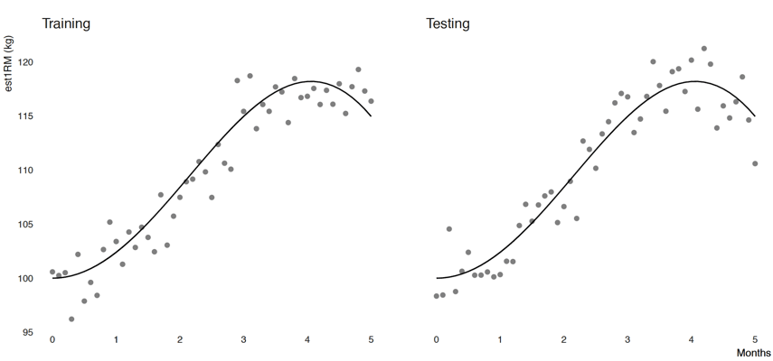
Figure 6.1. Simulated data. The black line represents the true 1RM, while the dots represent estimated 1RM using either LV profile or RIR equation. Data is split into training and testing. See text for further explanation

The black line on Figure 6.1 represent true 1RM across five months. As you can see, true 1RM rises up, plateaus shortly and drops. This can be due to change in training focus, dose or what have you. The dots around black line represent est1RM, and as you can see it doesn’t represent the perfect estimate of the 1RM. If est1RM is a perfect estimate of 1RM, it will lay over the black line. The data is split into training and testing, and as you can see, black lines are identical, but the dot’s vary due to measurement error.

Chapter 5 explained this using the following model:

Current Performance in this case would be est1RM, Stable Level of Adaptation would be true 1RM, and Current State + noise would be measurement error. Here it is as an equation:

The goal of the analysis would be to predict the true 1RM from the observed data (est1RM). The first model we are going to use is linear regression, but we will spice it up by adding polynomials. Let me explain.

The formula for a line is the following:

With the linear regression, we try to find the line (by finding coefficients  and ) that minimize the error. Here the error is represented as RMSE (root-mean-square-error) and represents the mean of the squared vertical distance between the line (model estimate or ) and the observed data (). To bring this error metric to a common scale, we take the root of this mean square error.

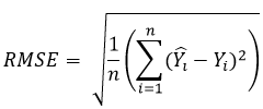
The smaller RMSE, the line fits better with the data. So we try to find the line that minimizes the RMSE. Since this is simulation, we know in advance that data is generated with RMSE of 2kg, which represents measurement error.

To spice this up, we can make this model more flexible by adding polynomials. The 2nd degree polynomial regression involves squaring X:

Third degree polynomial involve using x cubed:

The point is, the higher the polynomial degree, the more flexible the model and can fit the data better since it has more degrees of freedom or parameters to vary around. In other words we increase the model variance. Figure 6.2 contains the linear regression fit using training data with varying polynomial degrees (from 1 to 20).

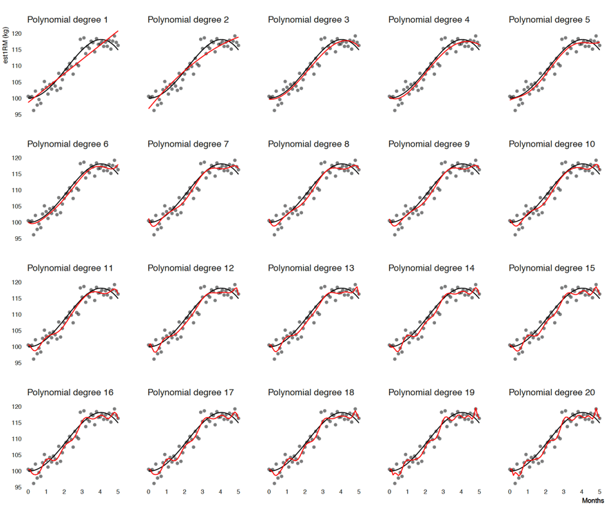
Figure 6.2. Linear regression fit using training data with varying polynomial degrees. Red line represents prediction, while black line represents true 1RM

Red line on Figure 6.2 represents linear regression prediction. As you can see, with increasing the polynomial degree, we are able to fit the model to the data better. In other words, higher the polynomial degree, lower the RMSE. For this particular model, polynomial degree represents model flexibility and a tuning parameter, that we can modify to find the best model fit or the model predictions.

To evaluate model predictive performance, one needs to use testing data (unseen hold-out sample) (James et al., 2017; Yarkoni & Westfall, 2017; Kuhn & Johnson, 2018). Figure 6.3 depicts predictive performance (using RMSE metric) for training and testing data set over different polynomial degrees.

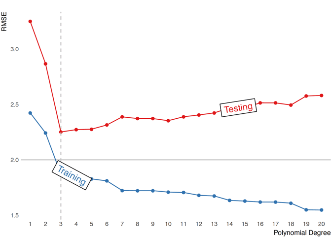
Figure 6.3. Predictive performance (using RMSE metric) for training and testing data set over different polynomial degrees. Horizontal line represents known measurement error which represents irreducible error. Vertical line represents the best polynomial degree that has the minimal RMSE for the testing data set, or in other words the best predictive performance.

Horizontal line on Figure 6.3 represents the known measurement error. This measurement error can be considered irreducible error³ (James et al., 2017). Models performing better than this irreducible error are overfitting – which means that they are modeling noise, not the signal. As can be seen from Figure 6.2, increasing polynomial degree improves performance of the model evaluated using the training data set. Model performs even better than the true irreducible error. But once the model performance is evaluated using unseen, testing data set, there is a fine line (indicated with the vertical dashed line) at which model performs the best. Everything to the right of the vertical line is overfit and everything to the left is underfit.

Vertical line also indicates optimal ratio between model bias and variance for this particular data set. Variance refers to the amount by which model parameters would change if we estimated it using a different training data set (James et al., 2017). On the other hand, bias refers to the error that is introduced by approximating a real-life problem, which may be extremely complicated, by a much simpler model (James et al., 2017). How are bias and variance estimated? One again needs to rely on the simulation, since in the simulation we can re-sample data from the known data generating process (DGP) (which is represented with the black line on figures 6.1 and 6.2). For a particular value of x, we have true value (black line), and also , which is predicted by the model. Over multiple simulations, for each particular model and tuning parameter (in this case polynomial degree) we can estimate the absolute error between true and , which represents bias, and variance in the in itself, which represents variance. This is done for every x value. The expected prediction error (MSE, which is same as RMSE but without root) for every x can be written as: