Strength Training Manual: Prescription – Part 3

1. Introduction
2. Agile Periodization and Philosophy of Training
3. Exercises – Part 1 | Part 2
4. Prescription – Part 1 | Part 2 | Part 3
5. Planning – Part 1 | Part 2 | Part 3 | Part 4 | Part 5 | Part 6

I am very happy to announce that I am finishing the Strength Training Manual. I decided to publish chapters here on Complementary Training as blog posts for two reasons. First, I want to give members early access to the material. And second, this way I can gain feedback and correct it if needed before publishing it.

I look forward to hearing your thoughts.

Enjoy reading!

How do we aggregate the training dose? What are the pros and cons of different dose metrics? How do we predict 1RM from training data? What is the “exertion load” metric, and why is it useful? How should the ballistic Load-Exertion table be adjusted? What are the simple heuristics for planning ballistic lifts and ‘quality reps’ in the grinding movements?

Find answers to these questions, and much more in Part 3 of the Prescription chapter.

Prediction and Monitoring

Before jumping to the strength training planning in Chapter 5, it is important to introduce few load (dose)¹ monitoring metrics that are commonly used, as well as to introduce few novel ones. As you will soon see, all these represent Small Worlds – or models with assumptions that attempt to represent Large World with a simple number. Nothing wrong with this of course. What is problematic is forgetting the distinction and trying to optimize the whole training based on few numerical aggregates. If you check the Figure 2.13 in Chapter 2, you can see that these data represent only one source of insight when making decision. Thus, they are needed and important, but just don’t forget that they represent an aggregated summary of a simplified Large World. It is very easy to fall for the Small World narrative of trying to optimize one metric to maximize training effects. The true story is that we do not know what variable drives (is associated or is causal) the training effects. Similarly, in a Kuhnian sense (Dienes, 2008), we do need to collect these studies and various models to push the scientific revolution forward, but the goal is not to become Intellectual Yet Idiot (IYI, to paraphrase Nassim Taleb) that sells this as objective ‘evidence-based’ approach. There is much more we do not know and that we do not capture with simple metrics.

Chapter 5 will expand more on the topic and the concept of load from a conceptual perspective, but in this chapter I will cover the most common metrics used to track the strength training load.

Table 4.24 contains 3 sets (8 reps at 73%, 6 reps at 79%, and 4 reps at 86%) with athlete subjective rating of exertion (RIR). I have provided a few summary metrics that I will explain below.

Table 4.24. Common training load summary metrics

Each set is summarized, and then at the bottom, the workout summary is provided. Here are the columns

Set – Indicate the order of the set.

Reps – Indicate how many reps has been planned/performed (here the assumption is that number of reps planned is equal to number of reps performed).

1RM – Represents athletes 1RM of the exercise (or EDM) used to estimate load.

%1RM – Percentage of the 1RM used.

Load – Calculated weight that needs to be lifted using athlete 1RM and %1RM of the program (Load = 1RM x %1RM).

RIR – Reps-In-Reserve. This is a subjective rating that athlete gives after the completion of the set.

The above variables represent the usual planning parameters (with the exception of RIR, that can be planned in advance and that can help in selecting the %1RM and reps, but it can also be subjective rating given by the athlete at the end of each set). The variable below are the aggregates or the summaries of each set.

NL– represent number of lifts (or reps). The summary at the bottom of the table represents simple sum

aRI– represents average relative intensity (%1RM) of the set. The summary at the bottom of the table can be calculated in two ways. First option (first number; 79%) is the simple average of three sets ((73% + 79% + 86%) / 3 = 79%). But we can also calculate it using reps, since each set contributed different number of reps to a grand summary. This is done using the weighted average where set percentage is multiplied by number of reps, and finally divided by NL. This is indicated by the second number (78%) and it is calculated the following way: (8 x 73% + 6 x 79% + 4 x 86%) / (8 + 6 + 4). As you will soon see, and I suggest you create an Excel workbook and play with the numbers, this is equal to Impulse / NL. With this very simple example, one can see the “Small World” model at hand – we immediately have the assumptions in the simple aggregate. You can also use average load metric, where instead of %1RM you use average weight.

Tonnage– Tonnage is a very common metric and it represents Reps x Load. The summary at the bottom of the table is a simple sum of tonnage of each set. Tonnage corresponds to mechanical work, but without the distance component.

Impulse– Impulse is relative tonnage. Imagine doing 3×5 @75% for bench press (1RM = 100kg) and deadlift (1RM = 200kg). Tonnage will be double for the deadlift since the higher absolute load used. Impulse is there to fix this issue and allow comparison between different exercises and individuals possible. Impulse is calculated by multiplying Reps x %1RM for each set, and the summary at the bottom of the table is the simple sum. A simpler way to calculate impulse is to use Tonnage / 1RM. Thus, impulse also tells you how many times you lifted your 1RM.

INOL– Intensity of Lift, is the metric created by Hristo Hristov (Hristov, 2005) to improve training prescription using the Prilepin Table. INOL is calculated by the following equation for every set: NL / (100 – 100 x %1RM). For example, set one (8 reps @73%) has INOL equal to 8 / (100 – 73), or 8 / 27, which is equal to 0.3. The summary at the bottom of the table is the simple sum of each set INOL. Hristov suggested the following training guidelines using INOL metric:

Table 4.25. Hristo Hristov guidelines for using INOL metric (Hristov, 2005)

All the above load metrics can be reported per intensity (%1RM) bracket rather than solely with the grand total. For example, one might be interested how many reps are done in the 80-90% range, what is the impulse in that range and so forth. It is always easy to get fancier with load metrics (for example you might calculate the work done using distances that barbell travel, or density using time to complete, which can be useful metric for some type of training, such as Mongoose Persistence or EDT – Escalatory Density Training (Staley, 2005)), but the objective is to be as simple as possible and get few actionable metrics. Having said this, I will contradict myself and introduce some novel metrics in a few paragraphs. To further understand why is this needed, consider the following examples.

The two metrics that are left are my invention and are more related to 1RM prediction and the estimate of proximity to 1RM than load:

pred1RM-Predicted 1RM is the equation already introduced. It is used to predict 1RM from load used, number of reps done and athlete RIR subjective rating:

1RM = (Weight x (Reps + RIR) x 0.0333) + Weight

This is a tool to track (embedded testing) effects – what is potentially happening to 1RM, without directly testing it (either with a true test, or with reps-to-failure). Please note that this prediction is based on Epley’s formula and subjective rating given by the athlete. For this reason it should be supplemented with something more demonstrable, such as plus set. Other options might involve predicted 1RM from load-velocity relationship (using 2-3 warm-up sets, e.g., 40-60-80%) and the known v1RM (velocity at 1RM) which can be personalized or group averaged. The goal here is not perfect prediction, but a gauge into trends over time that can supplement decision making after a training sprint or a phase.

prox1RM– Proximity to 1RM represent metric that estimates how close to 1RM a given set is. For example, if you do 5 reps with 100kg (regardless of RIR, since we are interested only in what is manifested), that would correspond to 1RM of (5 x 100 x 0.033) + 100, or 116.5kg. If your 1RM is equal to 130kg, then the ratio, or prox1RM is equal to 116.15 / 130, or 89%. This metric is useful to estimate how aggressive your are with your progressions (assuming no change in the pre-phase 1RM that we use to estimate loads). The higher the prox1RM, the more you are pushing it (will come back to this metric in Chapter 5 when discussing push the ceiling versus pull the floor approaches to planning strength training). Prox1RM is thus calculated:

prox1RM = ((Weight x Reps x 0.0333) + Weight) / 1RM

or using known %1RM

prox1RM = (%1RM x Reps x 0.0333) + %1RM

When you use known %1RM, rather than load, you can check the aggressiveness of your planning (given Epley’s formula). Thus, prox1RM is more of a planning tool, then monitoring tool. Table 4.26 contains calculated prox1RM using Load-Exertion table. The take home message is that lower the RIR, higher the prox1RM.

Table 4.26. Proximity to 1RM (prox1RM) calculated using Load-Exertion table

It is important to understand that all the metrics mentioned can be considered both as planning tools, as well as monitoring tools. This is pretty much related to before vs. after, and for this reason it might be interested to collect both, as planned vs. realized. This type of analysis can be done during the research and review phase and it can be quite insightful to figure out what works and what needs adjustment. When it comes to 1RM and all the metrics based on it, one can use pre-cycle 1RM (used to estimate the weight to be lifted), as well as to use pred1RM (either using the RIR or using velocity-based predictions) to adjust the metrics. For example, if you plan doing 3×5 with 80% and you use your 1RM which is 150kg, then the load you plan lifting is 120kg. Training load metrics, such as aRI, INOL, Impulse and all other, if bracketing technique is used (i.e. per intensity zone), use this 80% estimate. This is great for planning ahead and assuming pre-cycle 1RM (the one we used to establish weights) doesn’t change. But what if you feel really well on a particular day (which is normal variability in performance and thus 1RM) and your pred1RM shows 160kg? Then all the realized relative metrics will be off. Thus, it could be useful to use adjusted as well as as-planned load metrics (see Table 4.27). This can of course become major pain in the ass, so I recommend collecting the basic metrics, but reviewing and adjusting more frequently.

Table 4.27. Adding adjusted metrics based on realized performance (using pred1RM)

The long story short is that we need to differentiate between planned vs. realized load metrics. They can be adjusted based on performed training and using pred1RM, or it could be simpler than that using actually reps done by the athlete, and so forth. To make it simpler, I will assume they are equal from now on. Now let’s look at the following two example in Table 4.28 Try to spot the issues with contemporary load metrics:

Table 4.28. Two examples of set and rep schemes and contemporary load metrics. Can you spot the issues?

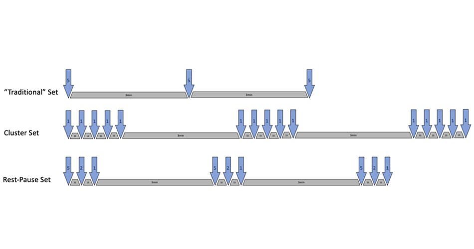
Table 4.28 gives two examples (1) 3 sets of 5 with 120kg but done at RIR 3 vs 1, and (2) 10×1 vs 1×10 with 150kg. With the exception of pred1RM and prox1RM, other load metrics give equal results for two different workouts in the two examples. Doing 3×5 with 150kg with 3RIR or 1RIR gives the same load metrics, which implies that proximity to failure is not taken into consideration with the current metrics. But we all bloody know that these two sets will create different stress on the lifter. Same thing with the second example: doing 1 set of 10, versus 10 sets of 1 gives equal load metrics results. Which brings me back to the “Small World” problem – these metrics are simplified and imperfect representations of the “Large World” complexities. Hence my pluralistic stance towards philosophy of science (see Chapter 1). Again, the problem is not using Small Worlds, but assuming they are objective truth and publishing using “Evidence-Based Approach”. Imagine (well you do not need to imagine) a bunch of lab coats trying to figure out the ‘optimal’ distribution of Small World metrics to minimize/maximize training effect and calling it ‘objective’ or ‘evidence-based approach’.

Well, enough of my rant on lab coats. The potential addition to the above metrics is to somehow rate reps differently based on how close to failure they are. Reps closer to failure (lower RIR) get more weight than reps done away(higher RIR) from failure. One such metric is called exertion load (XL), and it is being developed by Robert Frederick (Frederick, 2017, 2018). Figure 4.9 contains table and chart outlining non-linear weighting of the reps depending of how close they are to failure. The formula for weight is the following: