R Playbook: Injury Prediction using Random Forest
This is the problem I have been wrestling with for some time and I tried to solve it using Bannister model. I even asked for help on Twitter and couple of data scientists suggested taking a look into “functional data analysis” or creating summary variables and performing regression/classification (which I did here). Here is my Twitter post:
The problem I am looking for analyzing are predicting injury data for training load data. The basic structure involves multivariate time series (e.g. for every day and every player we track multiple training load metrics: training duration, distance covered, high intensity running and so forth – can reach >200 metrics) and TRUE/FALSE injury target variable (for occurrence) or days lost (for well – lost days). There are multiple ways to express “injury” occurrence/loss time, which I won’t go here.
What we are trying to do is to create injury risk/probability model for a single athlete (and/or team) from this multivariate time series data. I created a video I did using Banister model in analyzing very simple data set (single load metric), but failed to “constrain” injury probability with logit(stic) model. Here is the video: https://www.youtube.com/watch?v=7JqLafOR67Y
The problems are the following:
- I am trying to find a particular method in analyzing this data set – something that predicts from multivariate time series (just throwing things in regression will not help, since the order of data is important). Besides, if we change Injury target variable to performance (which is continuous), how can we predict one time series fro other multiple time series? Banister models works in this realm, but I am looking for other options (there is PerPot model by Perl).
- You need injuries to predict injuries. And some players don’t have them in the data set (which is good). So we need to use “hierarchical” model and try to make inferences on a individual from the group data (“Bayesian hierarchical” ?) e.g. apriori.
Any help with this is highly appreciate.
As I mentioned in the above post, I beleive that some type of Bayesian Hierarchical time-series analysis should be applied, but have no clue if such thing exists and how to apply it. So I tried to play with data summaries and performing more “traditional” approach (e.g. not time-series analysis).
For the sake of this playbook I will simulate some data for 60 athletes and 1000 days duration with couple of injuries. Since this is a lot of data, I will display only 100 data points for couple of athletes, but perform analysis on everyone.
Ok, let’s generate some data and display it in the table.
# Load libraries
library(randomNames)
library(dplyr)
library(ggplot2)
library(reshape2)
library(zoo)
library(rpart)
library(DMwR)
library(randomForest)
suppressPackageStartupMessages(library(googleVis))

# Generate data
set.seed(100)
numberOfPlayers <- 60
numberOfDays <- 1000


playersData <- data.frame(Name = rep(randomNames(numberOfPlayers, which.names = "first"), numberOfDays),
                          Day = rep(1:numberOfDays, each = numberOfPlayers),
                          Load = runif(numberOfPlayers * numberOfDays, min = 0, max = 100))

playersDataPrint <- playersData %>%
                    filter(Day > 300,
                           Day < 400,
                           Name == "Alec" | Name == "David" | Name == "Emily" | Name == "William" )
Here is the same data plotted:
# Plot the data
gg <- ggplot(playersDataPrint, aes(x = Day, y = Load)) +
    geom_bar(stat = "identity", fill = "#8C8C8C", alpha = 0.6) +
    facet_wrap(~Name) +
    theme_bw()
gg
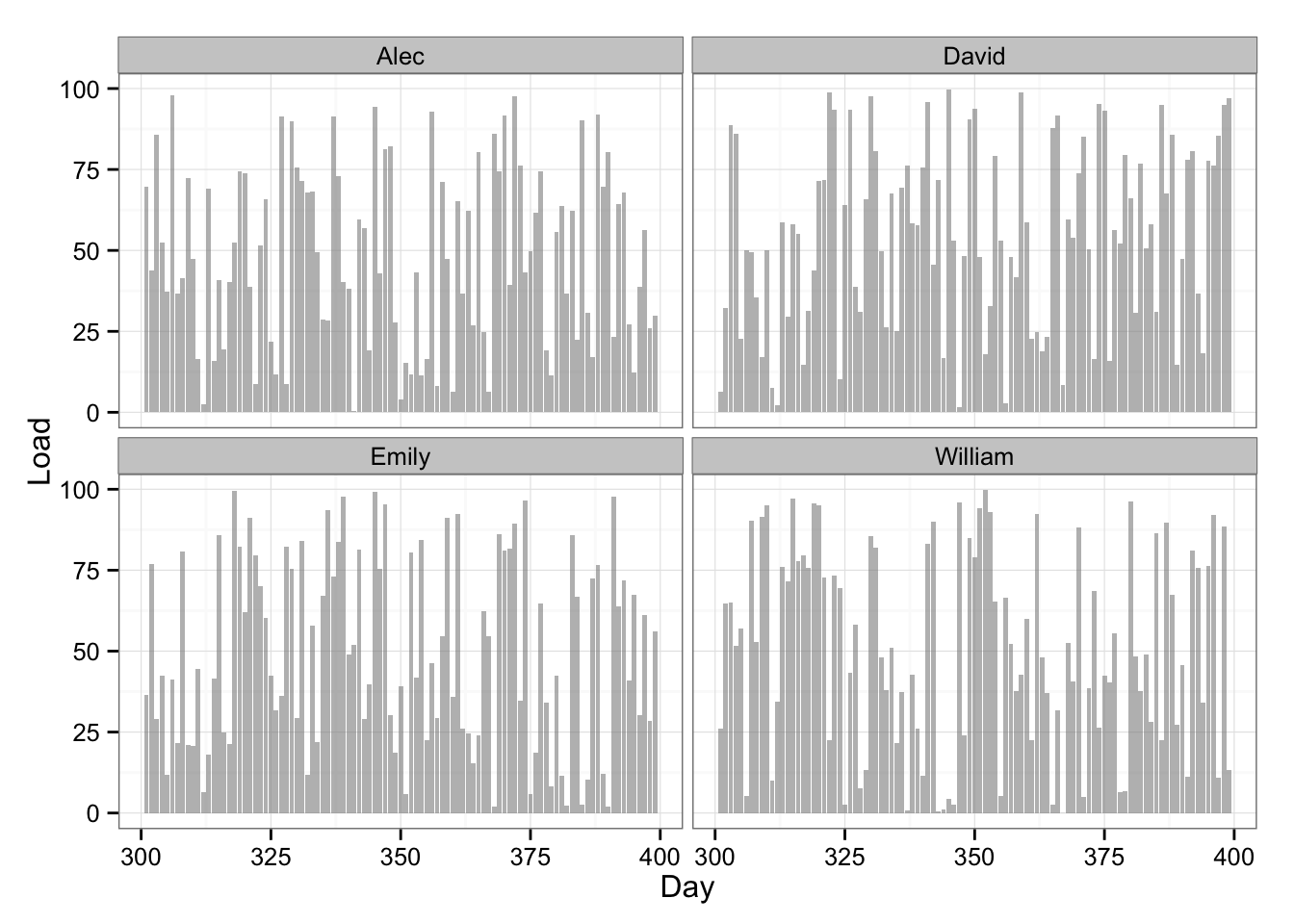
What we need to do now is to create some summary metrics. I decided to do 7,14,21,28,35,42 rolling averages/sum/sd for each athlete. I started using dplyr package which is great for data wrangling
# Engineer the metrics
for (summaryFunction in c("mean", "sd", "sum")) {
    for ( i in seq(7, 42, by = 7)) {
        tempColumn <- playersData %>%
                      group_by(Name) %>%
                      transmute(rollapply(Load,
                                          width = i,
                                          FUN = summaryFunction,
                                          align = "right",
                                          fill = NA,
                                          na.rm = T))
        colnames(tempColumn)[2] <- paste("Rolling", summaryFunction, as.character(i), sep = ".")
        playersData <- bind_cols(playersData, tempColumn[2])
    }
}
Since rolling data summaries will leave NAs for rows which rolling window doesn’t take into consideration, I decided to trim our data to leave out NAs.
# Cut out first 100 days to avoid NAs in RandomForest later
playersData <- playersData %>%
                filter(Day > 100) %>%
                mutate(Day = Day - 100)

# Create shorter data frame for visualizing
playersDataPrint <- playersData %>%
                    filter(Day > 300,
                           Day < 400,
                           Name == "Alec" | Name == "David" | Name == "Emily" | Name == "William" )
Here is the table of the data and plot with 7 and 42 rolling average:
# Plot the data with two rolling averages
gg <- ggplot(playersDataPrint, aes(x = Day, y = Load)) +
    geom_bar(stat = "identity", fill = "#8C8C8C", alpha = 0.6) +
    geom_line(aes(y = Rolling.mean.7, x = Day), color = "#5DA5FF", size = 1) +
    geom_line(aes(y = Rolling.mean.42, x = Day), color = "#60BD68", size = 1) +
    facet_wrap(~Name) +
    theme_bw()
gg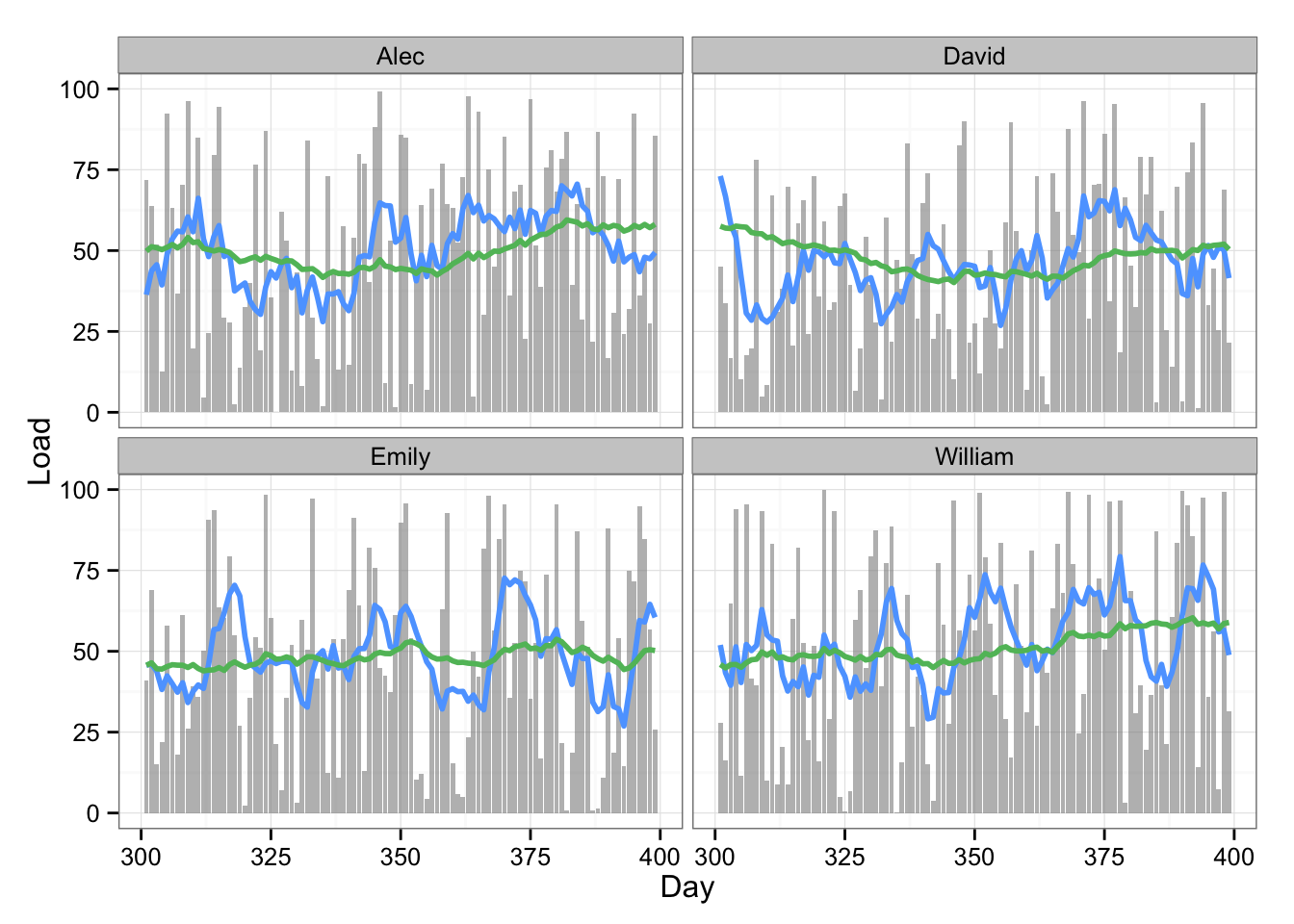
The 7 and 42 rolling averages quickly give us some glimpse into what is happening with training load. As one can see from the table, we quickly create numberous summary variables from a single load metric. Since there can be multiple load metrics (or anything else we keep track of, like HRV, jump performance, etc) the number can reach big number quickly.
Now we need to create injury occurence. We need “taget” variable tha I have calles “Status” which can have two states “Available” and “Injured”. When injury happens, we tag it only once (without the information about the time loss and duration of the injury, which could be another variable). Since this is “binary” target variable, we are basically dealing with “classification” issues. Taking into account the above huge number of predictors, the logistic regression is not the best choice since we need to select metrics that are predictive. Instead we need to use Decision Trees and Random Forest that select important metrics automatically.
Anyway, I decided to tag injury when different rolling loads reach certain threshold. I also had to be sure to tag it only once. Of course, the training load will drop after injury, but for the sake of an example I didn’t change the load after the injury.
# Generate injury variable
playersData <- playersData %>%
                mutate(Status = ifelse((playersData$Rolling.mean.42 > 55) &
                                 (playersData$Rolling.mean.7 > 75) &
                                 (playersData$Rolling.sd.42 < 35),
                                "Injured", "Available")) %>%
                mutate(Status = replace(Status, is.na(Status), "Available"))

playersData$Status <- factor(playersData$Status, levels = c("Available", "Injured"))

# Delete repeated Injury status - keep only one
playersData <- playersData %>%
                group_by(Name) %>%
                mutate(prev = lag(Status)) %>%
                mutate(Status = replace(Status,
                                        Status == "Injured" & prev == "Injured",
                                        "Available")) %>%
                select(-prev)

# Create shorter data frame for visualizing
playersDataPrint <- playersData %>%
                    filter(Day > 300,
                           Day < 400,
                           Name == "Alec" | Name == "David" | Name == "Emily" | Name == "William" )
Here is the plot with injury data
# Plot the data with two rolling averages and status
gg <- ggplot(playersDataPrint, aes(x = Day, y = Load)) +
    geom_bar(stat = "identity", alpha = 0.6, aes(fill=Status)) +
    scale_fill_manual(values=c("#8C8C8C", "#F15854")) +
    geom_line(aes(y = Rolling.mean.7, x = Day), color = "#5DA5FF", size = 1) +
    geom_line(aes(y = Rolling.mean.42, x = Day), color = "#60BD68", size = 1) +
    facet_wrap(~Name) +
    theme_bw()
gg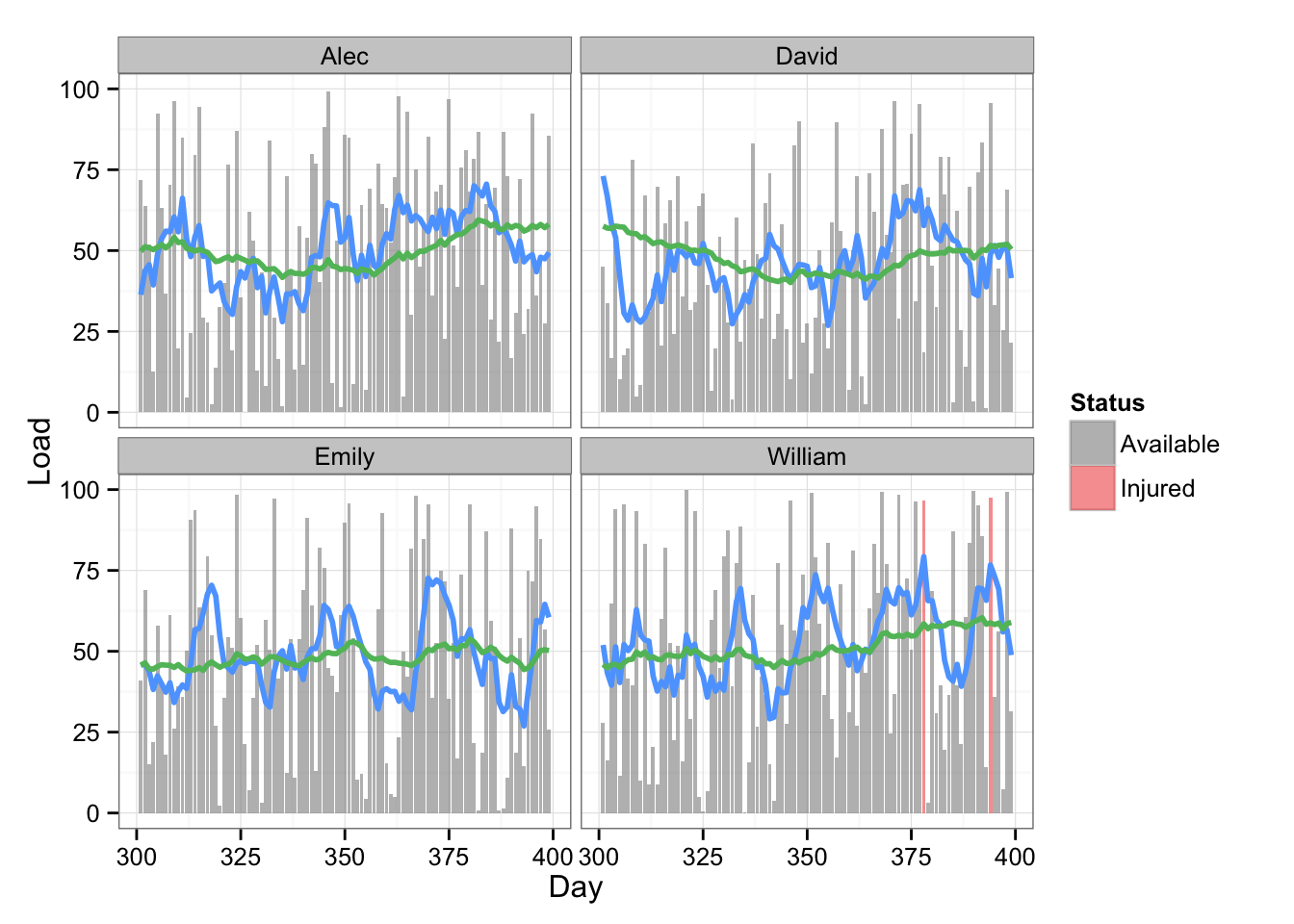
And the boxplots for every variable
# Box plots for every variable
playersDataLong <- melt(playersData, id.vars = c("Name", "Day", "Status"))

gg <- ggplot(playersDataLong, aes(Status, value)) +
    geom_boxplot(alpha = 0.8, aes(fill=Status)) +
    scale_fill_manual(values=c("#8C8C8C", "#F15854")) +
    facet_wrap(~variable, scales = "free") +
    theme_bw()
gg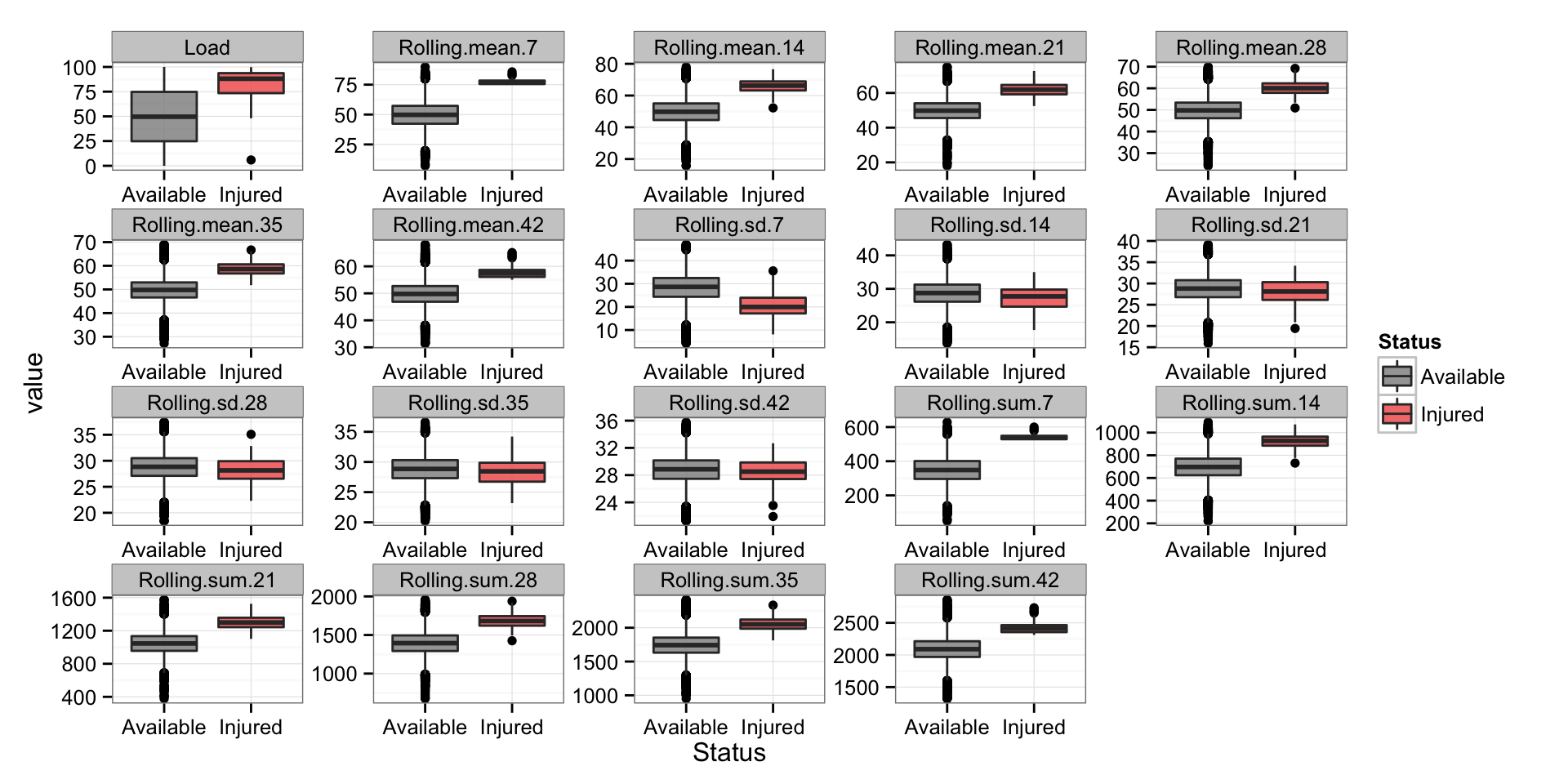
I have also performed Principal Components Analysis to visualize this multidimensional data and also color code the injury rows to see if there are any clusters forming.
# PCA (color = status)
playersDataNormal <- as.data.frame(scale(playersData[3:21]))
PCA <- prcomp(playersDataNormal)

PCA.plotting <- cbind(playersData[22], PCA$x[,1:2])

gg <- ggplot(PCA.plotting, aes(x = PC1, y = PC2, color = Status, shape = Status)) +
    geom_point(alpha = 0.7) +
    scale_color_manual(values=c("#8C8C8C", "#F15854"))+
    theme_bw()
gg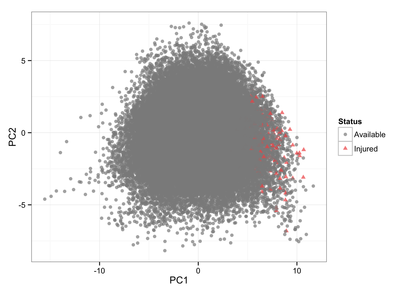
And now I am going to perform Regression Tree to see if we can predict injury occurence from summary variables. I am not going to deal with cross validation, but will only simply create model on all data set and present the graph and confusion matrix
# Regression Tree


model1 <- rpartXse(Status ~., playersData[-(1:2)])
prettyTree(model1)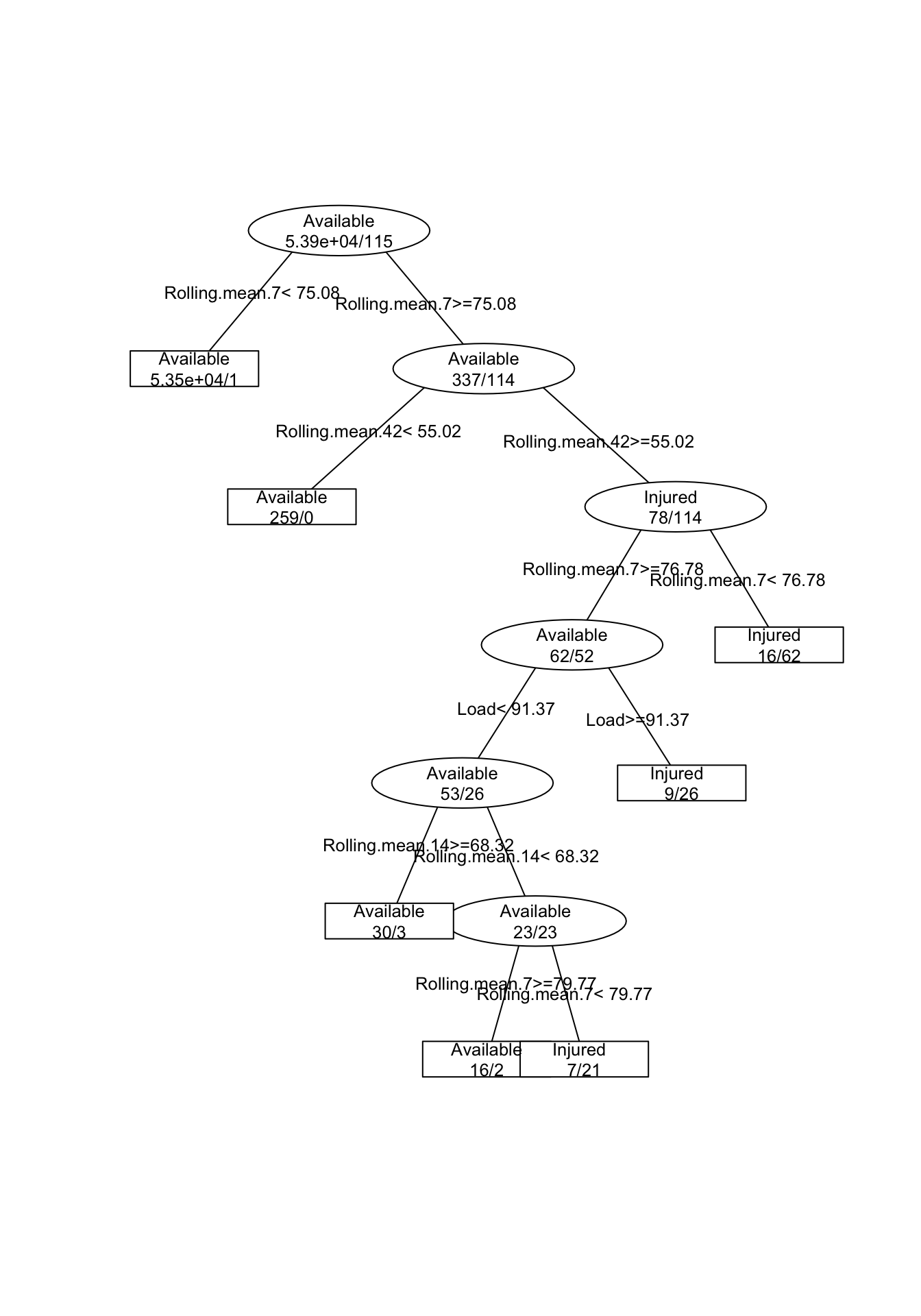
# Confuction matrix
predicted.injury <- predict(model1, type = "class")
table(playersData$Status, predicted.injury)
## predicted.injury
## Available Injured
## Available 53853 32
## Injured 6 109The next step is to use Random Forest, check what variables are the most predictive, get the confsion matrix and plot the predictions
model2 <- randomForest(Status ~.,
                       playersData[-(1:2)],
                       ntree = 1000,
                       importance = TRUE)
varImpPlot(model2, type = 1)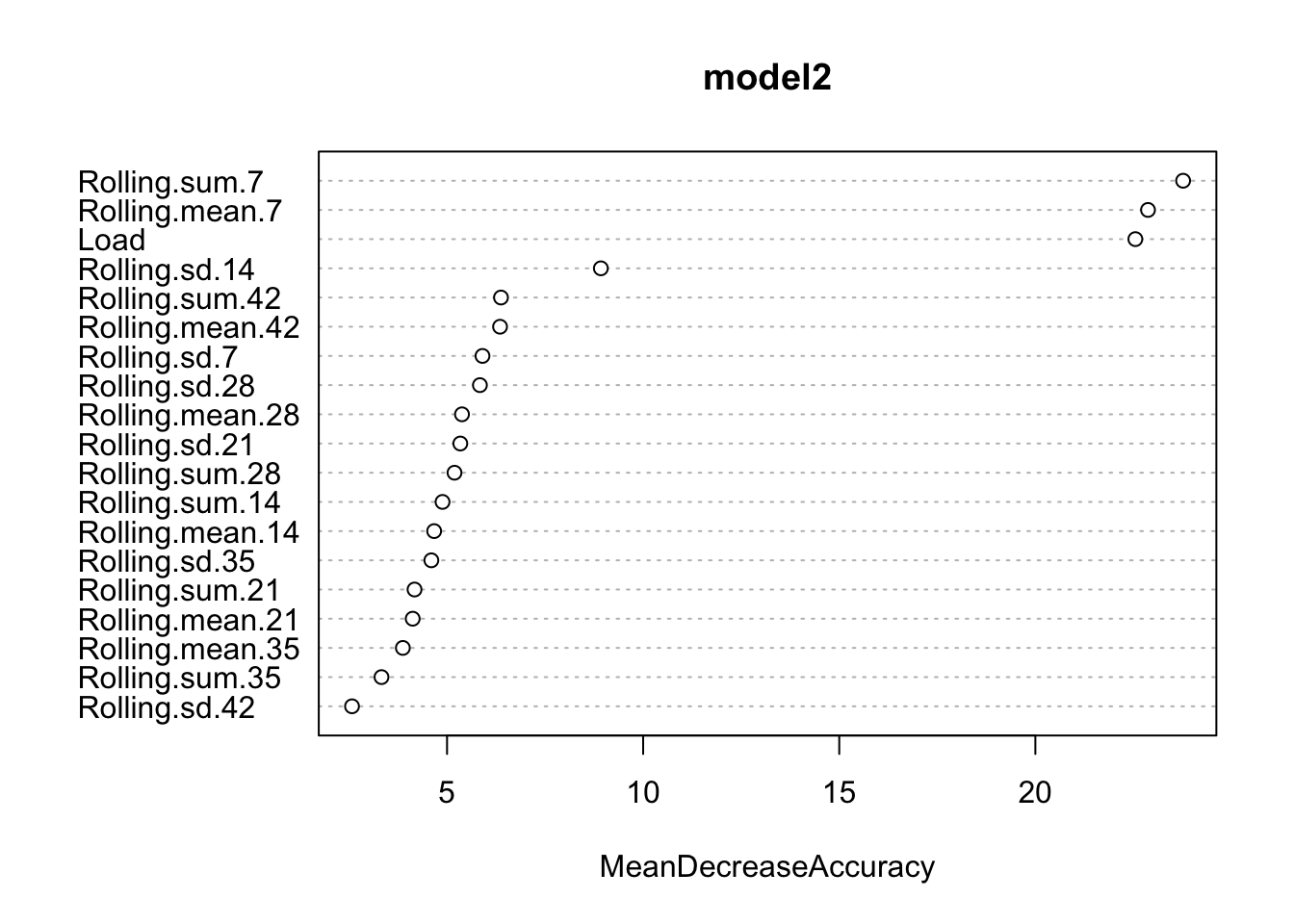
# Predict the injury
playersData$Injury.Pred.Prob <- predict(model2, type = "prob")[,2] * 100
playersData$Injury.Pred.Class <- predict(model2, type = "class")

# Confusion matrix
table(playersData$Status, playersData$Injury.Pred.Class)
##
## Available Injured
## Available 53857 28
## Injured 29 86# Create shorter data frame for visualizing
playersDataPrint <- playersData %>%
filter(Day > 300,
Day < 400,
Name == "Alec" | Name == "David" | Name == "Emily" | Name == "William" )
# Plot the predictions
gg <- ggplot(playersDataPrint, aes(x = Day, y = Load)) +
geom_bar(stat = "identity", alpha = 0.6, aes(fill=Status)) +
scale_fill_manual(values=c("#8C8C8C", "#F15854")) +
geom_line(aes(y = Injury.Pred.Prob, x = Day), color = "#F15854") +
facet_wrap(~Name) +
theme_bw()
gg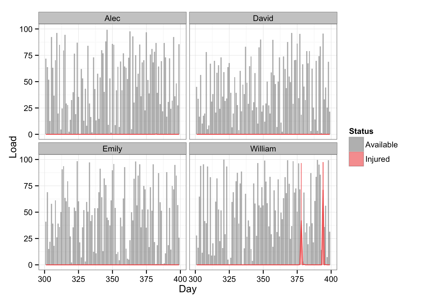
We can compare two confusion matrix and set up the predicion threshold to reach different “false positive” and “false negative” percentages.
As I said I won’t go into cross valiadation here. What is interesting to note is that we can “match” the injured players, and instead plugging everything into the analysis we can pull N closest neighbours. The # of closest neighbours could be considered “tuning” parameter. I guess that this could give us more “graded” probabilities as opposed to current solution. Definitely something to play with.
Anyway, with the method above we used all of our data to get injury prediction. But in my opinion the next step is to create models for every person. Implementing some type of multilevel/hierarchical regression has to be the way to do it. Unfortunatelly I am not very versed in this area.
Hope this short playbook gives you some ideas on how to use Random Forest for injury prediction.



Responses