Optimal Force-Velocity Profile for Sprinting: Is It All Bollocks?

In the next two parts of this article series I will explain how the optimization of the Force-Velocity Profile (FVP) works. Before jumping into FVP optimization, I will explain the same reasoning using the Acceleration-Velocity Profile (AVP) first, since it is easier to comprehend.

It is important to re-emphasize again that we are working with the model (Figure 1). As you will see, optimization is a form of model sensitivity analysis: pretty much, we are playing with the parameters to check how the model responds in its predictions (Figure 2).

Figure 1: Small World is just a map of the Large World (“Terrain”)

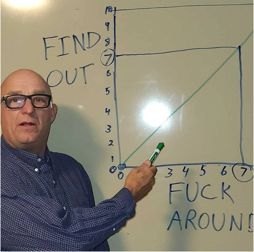
Figure 2: Model sensitivity is just “fuck around and find out”

Optimization of the Acceleration-Velocity Profile

Let’s imagine we have an athlete with MSS (maximum-sprinting-speed) equal to 9 $ms^{-1}$ and MAC (maximum-acceleration) equal to 8 $ms^{-2}$. These are model parameters that we will use to generate the data (again, we are using model predictions). These parameters gives us TAU of 1.125 $s$ and $P_{max}$ equal to 18 $W/kg$.

Using Equation 1 and these known parameters, we can predict times at different distances (i.e., split times) without problems.

\begin{split}
t(d) = TAU \times W(-e^{\frac{-d}{MSS \times TAU}} – 1) + \frac{d}{MSS} + TAU
\\\end{split}Equation 1

Table 1 contains model predicted split times using aforementioned parameter values.

Show/Hide Code


require(tidyverse)
require(shorts)
require(cowplot)
require(directlabels)
require(kableExtra)

athlete_MSS <- 9
athlete_MAC <- 8

split_times <- tibble(distance = c(5, 10, 15, 20, 25, 30, 35, 40, 45)) %>%
  mutate(
    time = predict_time_at_distance(distance, athlete_MSS, athlete_MAC)
  )

kbl(split_times, digits = 2) %>%
  kable_classic(full_width = FALSE)

distance	time
5	1.34
10	2.06
15	2.69
20	3.29
25	3.87
30	4.44
35	5.00
40	5.56
45	6.12

Table 1: Model predicted split times for athlete with MSS equal to 9 m/s and MAC equal to 8 m/s/s

Now that we have this generative model in our hands, we can play with the parameters to check model predictions. In other words, we are performing model sensitivity analysis. Even simpler, we are doing what-if analysis. For example, how will our times per distance decrease if we improve MSS or MAC parameter for certain percentage.

I have called this type of analysis probing, and you can see the results in Figure 3. I will introduce one more type of sensitivity analysis later on (the one actually utilized by Samozino et al. (2022)), but probing is more intuitive to comprehend and will serves us a nice foundation.

Show/Hide Code


# Generate data
model_sens_df <- tibble(MSS = athlete_MSS, MAC = athlete_MAC) %>%
  expand_grid(
    distance = seq(5, 45, by = 5),
    increase = c("MSS", "MAC"),
    factor = seq(100, 120)) %>%
  mutate(
    distance_label = factor(paste(distance, "m"), levels = paste(seq(5, 45, by = 5), "m")),
    increase = factor(increase, levels = c("MSS", "MAC")),
    time = predict_time_at_distance(distance, MSS, MAC),
    new_MSS = ifelse(increase == "MSS", MSS * factor / 100, MSS),
    new_MAC = ifelse(increase == "MAC", MAC * factor / 100, MAC),
    new_time = predict_time_at_distance(distance, new_MSS, new_MAC),
    time_diff = new_time - time,
    time_perc_diff = -time_diff / time * 100
  )

# Plot
ggplot(model_sens_df, aes(x = factor - 100, y = new_time, group = distance_label)) +
  theme_linedraw(8) +
  geom_line(alpha = 0.6, color = "dark blue") + 
  geom_dl(
    aes(label = paste("  ", distance_label)),
    method = list("last.bumpup", cex = 0.5)
  ) +
  facet_wrap(~increase) +
  ylab("Time (s)") +
  xlab("Parameter Improvement (%)") +
  xlim(0, 22.5)

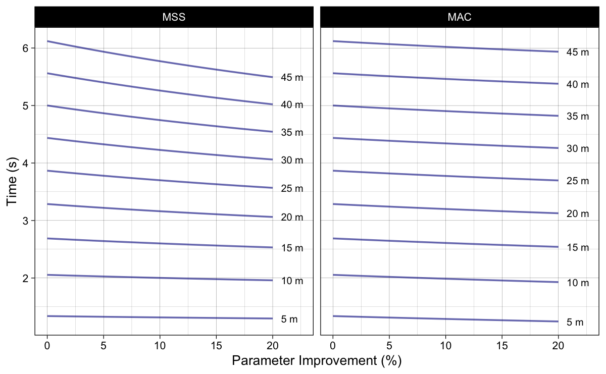
Figure 3: Model predicted split times when parameters are improved for certain percentage

Rather than showing predicted split times, we can show how much original split times improve. This can be done by calculating time difference ($\Delta t = t_{new} – t_{orig}$), or as shown in Figure 4, by calculating percent improvement, which is equal to $-100 \times \frac{\Delta t}{ t_{orig}}$. Please note that I have changed the sign of the percent improvement to be positive for easier graph reading (i.e., higher improvement, better split times).

Show/Hide Code


ggplot(model_sens_df, aes(x = factor - 100, y = time_perc_diff, group = distance_label)) +
  theme_linedraw(8) +
  geom_abline(slope = 1, linetype = "dotted", color = "dark grey") +
  geom_line(alpha = 0.6, color = "dark blue") + 
  geom_dl(
    aes(label = paste("  ", distance_label)),
    method = list("last.bumpup", cex = 0.5)
  ) +
  facet_wrap(~increase) +
  ylab("Time improvement (%)") +
  xlab("Parameter Improvement (%)") +
  xlim(0, 22.5) 
  #ylim(-0.7, 0.2)

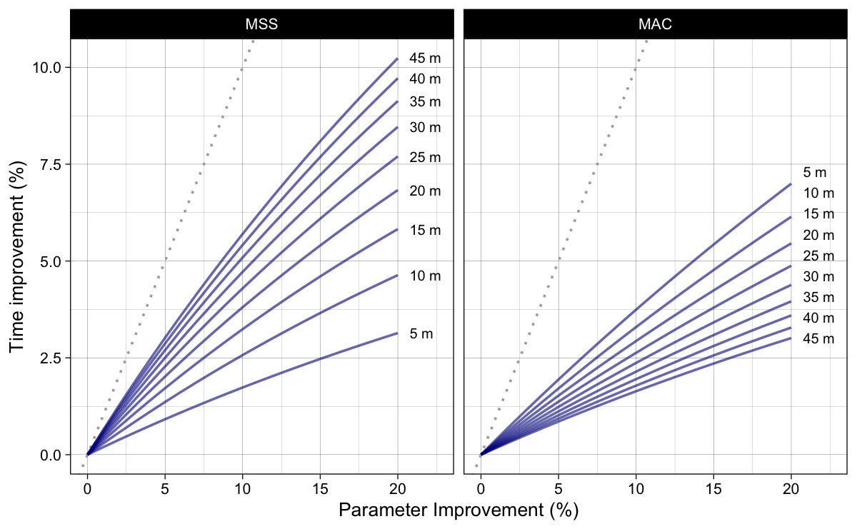
Figure 4: Model predicted split time improvements (in percentage) when parameters are improved for certain percentage. Dottel line represent identity line (i.e., slope 1)

The question that naturally follows the analysis from Figure 4 is “improving which model parameter yield higher time improvements?”. We can plot the data in a slightly different format to allow us to answer that question, as depicted in Figure 5. What we can see, is that improving MAC yields higher time improvements for distances < ~15m, while improving MSS yields higher time improvements for distances > ~15m.

Show/Hide Code


ggplot(model_sens_df, aes(x = factor - 100, y = time_perc_diff, color = increase)) +
  theme_linedraw(8) +
  geom_abline(slope = 1, linetype = "dotted", color = "dark grey") +
  geom_line(alpha = 0.6) + 
  geom_dl(
    aes(label = paste("  ", increase)),
    method = list("last.bumpup", cex = 0.5)
  ) +
  facet_wrap(~distance_label) +
  ylab("Time improvement (%)") +
  xlab("Parameter Improvement (%)") +
  xlim(0, 25) +
  #ylim(-0.7, 0.1) +
  scale_color_brewer(palette = "Set1") +
  theme(legend.position = "none")

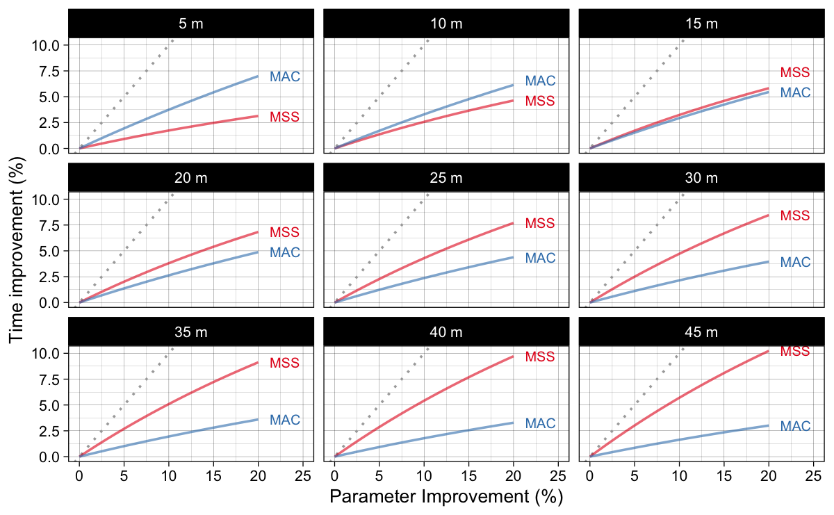
Figure 5: Model predicted split time improvements (in percentage) when parameters are improved for certain percentage. This figure answers “improving which model parameter yield higher time improvements?” question

Warning before we move on

You might be eager to conclude, based on Figure 5 that to improve <10m sprint times you are better off improving your maximum acceleration, while to improve…