Workbook: Change Point Analysis of HRV Data
I have already wrote about time-series analysis in EXCEL (HERE and HERE ) using Andrew Flatt HRV data. What I will try to do in this post is to use something that is called Change Point Analysis or CPA. This could be used with any type of time-series data, like training load, wellness and readiness monitoring and so forth.
I haven’t found much instructions online nor in books on CPA, but I have used this article to play with Andrew Flatt data. When it comes to time-series analysis there is great chapter in Data Smart book by John Foreman, which is a must read book for anyone willing to explore data analysis. There are also a free booklet (which I haven’t read yet) on time-series analysis in R here and Introductory Time Series with R book that could be worth checking.
Anyway, without going into intricate and unnecessary details of CPA, the simple goal for sport scientist using CPA is to detect changes in time-series data.
Let’s get rolling. First I will load HRV data from CSV file and load neccessary packages:
#install.packages("changepoint")
library("changepoint")

# Load data
HRV.Data <- read.csv(file = "Andrew Flatt HRV.csv", header = TRUE)
Andrew took HRV almost daily (I say almost since there are some missing days, but for the sake of an example I will assume daily measures, because I don’t know how to deal with missing values at this point) for over a year (399 observations to be exact). Let’s perform CPA and plot the results:
mvalue = cpt.meanvar(HRV.Data$HRV, method="BinSeg")
plot(mvalue,
     main = "Andrew Flat HRV",
     xlab = "Days",
     ylab = "HRV")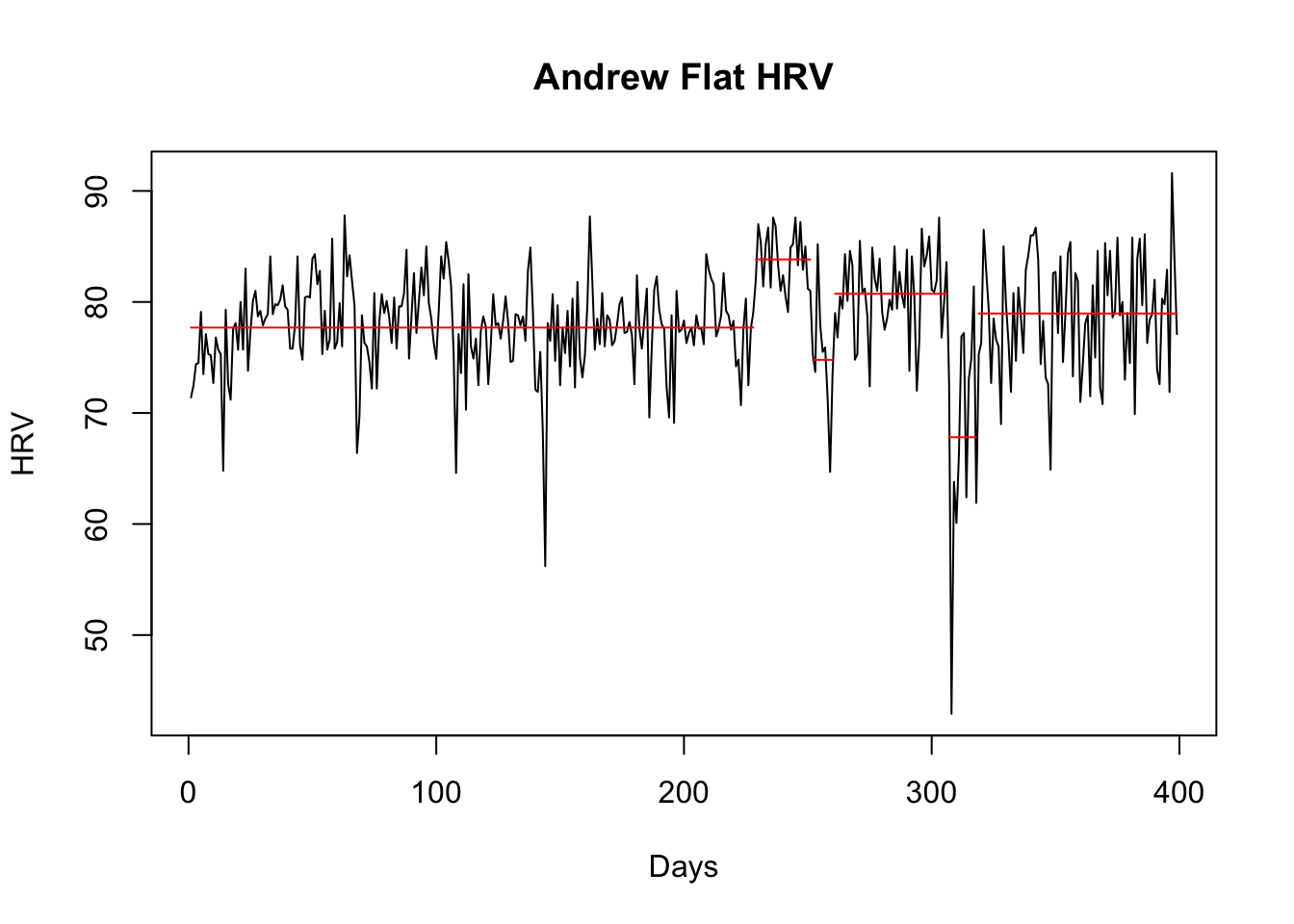
One can always play with CPA parameters and methods, but I will not do it now (because it it beyond my understanding at this point). What we immediately see are certain “blocks” that might indicate changes in training, lifestyle, etc that reflects changes in HRV.
We will do same for rest HR:
mvalue = cpt.meanvar(HRV.Data$HR, method="BinSeg")
plot(mvalue,
     main = "Andrew Flat rest HR",
     xlab = "Days",
     ylab = "Rest HR")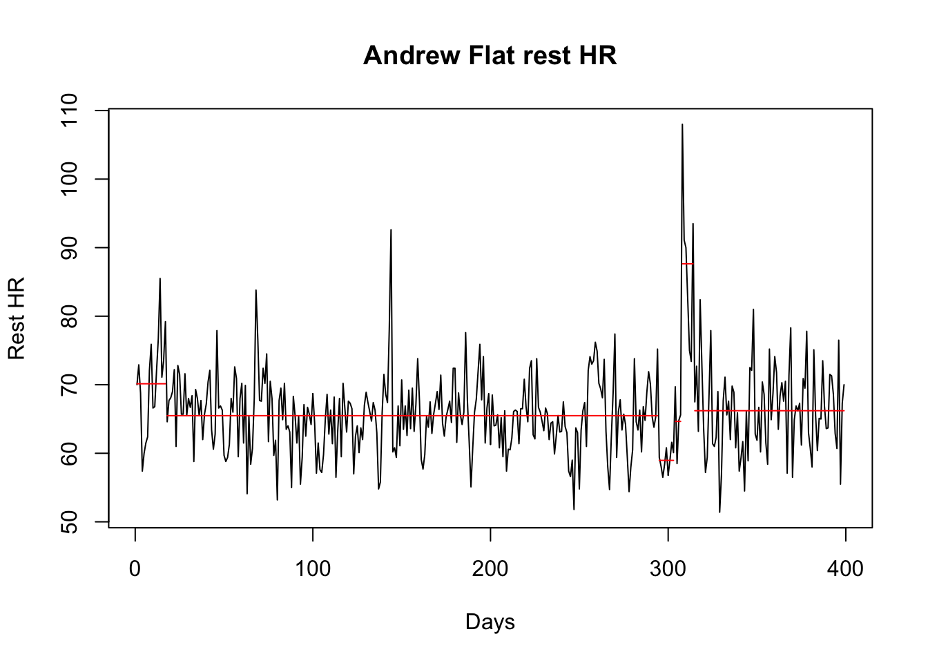
And for the ratio between HRV and HR (which is used to show saturation or something like that, can’t remember now and can’t be bothered to search in Martin Buchheit papers):
HRV.Data$HRV.HR.Ratio <- HRV.Data$HRV / HRV.Data$HR
mvalue = cpt.meanvar(HRV.Data$HRV.HR.Ratio, method="BinSeg")
plot(mvalue,
     main = "Andrew Flat rest HRV/HR",
     xlab = "Days",
     ylab = "HRV/HR")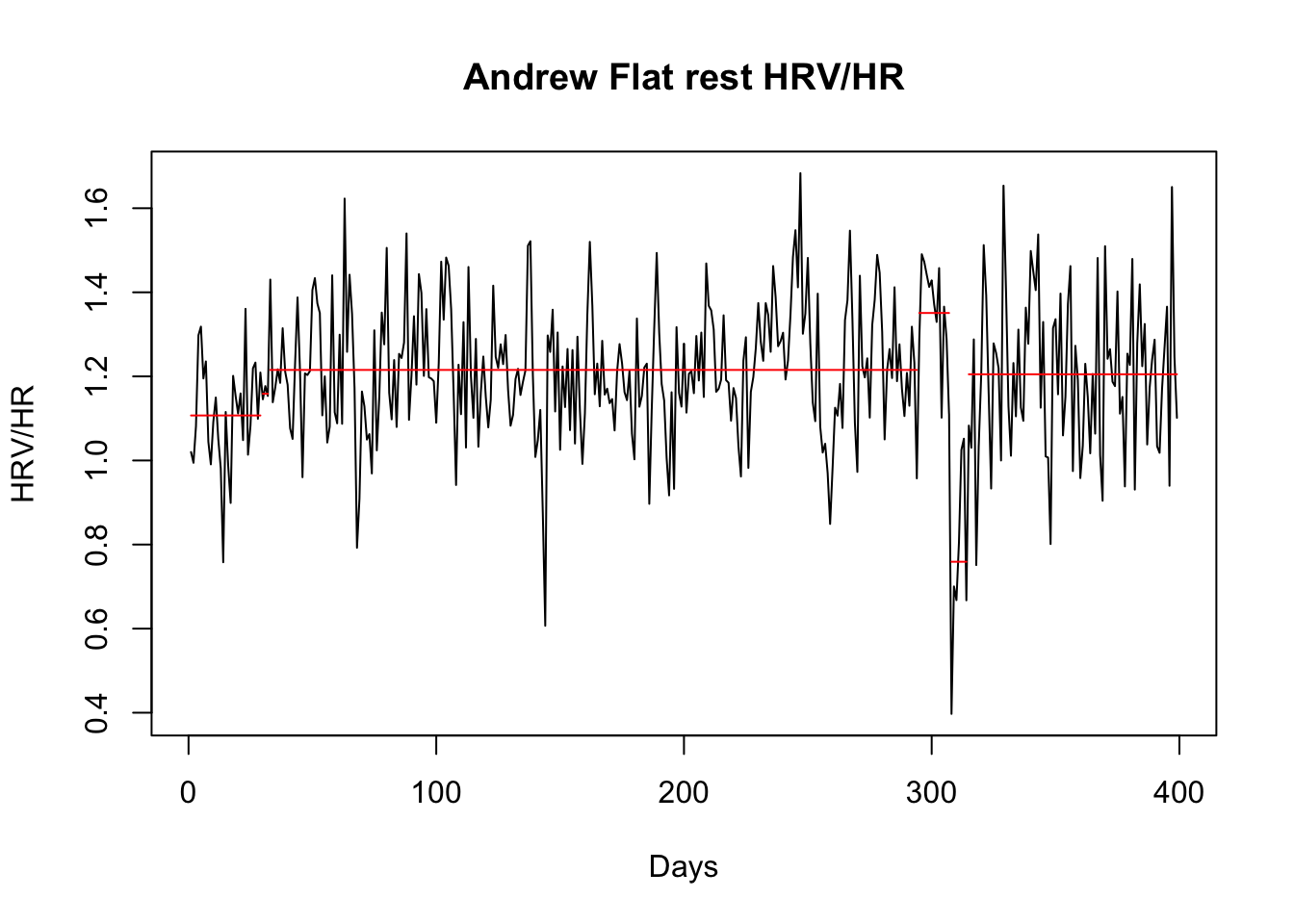
As with any model and analysis it is important to check the model fit and adjust the model parameters. Since this is the first time I am using CPA I have no clue how to do it.
When it comes to the above results I will leave Andrew to comment on what these might represent to him.
I will try to expand further on these methods in the future, but I first need to read and re-read the above mentioned resources. Too much books, too little time and data analysis is a rabbit hole.


Responses