Strength Training Manual Planning – Part 2

1. Introduction
2. Agile Periodization and Philosophy of Training
3. Exercises – Part 1 | Part 2
4. Prescription – Part 1 | Part 2 | Part 3
5. Planning – Part 1 | Part 2 | Part 3 | Part 4 | Part 5 | Part 6

I am very happy to announce that I am finishing the Strength Training Manual. I decided to publish chapters here on Complementary Training as blog posts for two reasons. First, I want to give members early access to the material. And second, this way I can gain feedback and correct it if needed before publishing it.

I look forward to hearing your thoughts.

Enjoy reading!

Dose -> Response

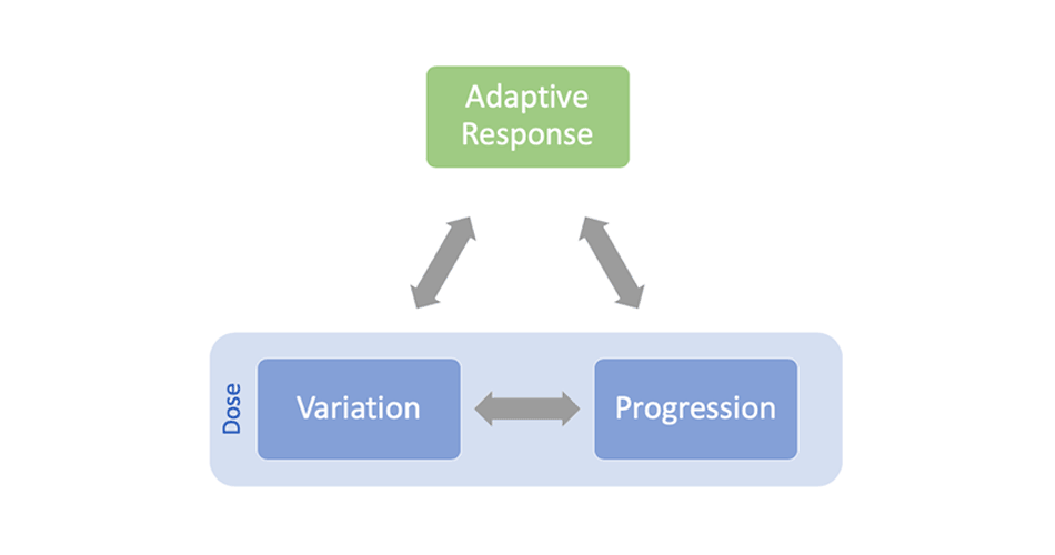
So far I have discussed dose as an independent construct and hopefully, from the previous pages you could get a glimpse of how the concept of dose is very complex and can be expressed in multiple and interacting ways. The “Small World” models that follow assume dose as a simple construct that represents some type of  stress or a stimuli that produces an adaptive response (Figure 5.11). This adaptive response is also a construct which can represent a multitude of responses, both in quality and quantity. Keep in mind that this and other “Small World” models that follow are simplistic representations of much more complex “Large World”.

Figure 5.11. Dose – Response model. Dose is a stress or stimuli that produces adaptive response.

Simple pharmacological model

Using a simple theoretical pharmacological model, depending on the response it produces, dose can have a range between the minimum effective dose (MED) and the maximum tolerated dose (MTD) (Figure 5.12). This is from Wikipedia (“Effective dose (pharmacology),” 2019):

The MED is defined as the lowest dose level of a pharmaceutical product that provides a clinically significant response in average efficacy, which is also statistically significantly superior to the response provided by the placebo. Similarly, the MTD is the highest possible but still tolerable dose level with respect to a pre-specified clinical limiting toxicity. In general, these limits refer to the average patient population. For instances in which there is a large difference between the MED and MTD, it is stated that the drug has a large therapeutic window. Conversely, if the range is relatively small, or if the MTD is less than the MED, then the pharmaceutical product will have little to no practical value.

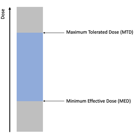
Figure 5.12. Dose can have a range between the minimum effective dose (MED) and the maximum tolerated dose (MTD). Of course, dose can go higher or lower than these thresholds, but the downside is significant in that case.

Dose zones

This dose range is usually qualitatively split into (1) restoration or recovery zone, (2) retention or maintenance zone, and (3) development zone. Table 5.7 contains an example of such a split from Vladimir Issurin books (Issurin, 2008, 2013, 2015). Please note that these zones (including MED and MTD thresholds) are pretty hard to pinpoint or estimate exactly, but as a concept they represent theoretical constructs which could be an interesting sandbox model. Later in this chapter I will introduce my own “forum for action” model, that I believe is more suited to uncertain context and complex interactions between different doses, specificities, densities and so forth (which all affect the dose and these thresholds/zones). But more about it in a few pages. Let’s now cover this conceptual model in more detail.

Table 5.7. Classification of the training dose. Modified based on Vladimir Issurin (Issurin, 2008, 2013, 2015)

Restoration zone is conceptual dose that is below MED, whose aim is to provide an active recovery to speed up the recovery processes¹. I personally think this is bullshit. I have been swallowing this theoretical story for years, but now I think slightly different. Let me expand. There is a belief that you can speed up recovery by performing some type of restorative work (dose, or means and methods). Not sure you can though – sleeping, eating, reducing stress (e.g., work related, school related and so forth) and probably providing variety for the sake of mental and emotional break is what might “work”. I do not think that by performing some activity in the “recovery” zone improves recovery. What I do believe is that one can perform whatever one can (and should) perform with quality at a given state of the organism and recovery that propels someone forward. This might be another means and methods with the retention/developmental dose that doesn’t dig a deeper recovery hole. For example, when someone is tired from say German Volume training (10×10) of squats and sore as fuck one day, doing squats the next day in the restoration zone (whatever that zone might be) will not bloody help restoration. What needs to be done in this case is answering the following question: “What other type of quality can I develop while I feel like shit, that doesn’t impair natural recovery processes?”. The answer might be in particular order: upper body work, core, low back rehab, small stabilizing muscles work, stretching or just chilling in the pool to get a mental break from training, eating pizza, banging and watching your favorite TV shows. Even better, you might figure out that you screw yourself over with pushing too much the previous day. In plain English, you do not do stuff to speed up recovery, but do stuff that can be done at that state and work “around” fatigue without imposing additional stress or digging yourself in the deeper hole.

Retention zone is very similar to minimum effective dose (MED) with a small caveat – retention dose is the dose that is needed to maintain (or retain) current level of a given quality, where MED is the dose that produce smallest practical change in a particular quality. Thus, retention zone is below MED threshold. I called it Minimum Retention Dose (MRD).

Development zone is between MED and MTD. It is thus a big area that can be further divided.

Upside and Downside effects (responses)

Development zone is usually split into multiple sub-zones (see Table 5.7 for an example). This is because response involves both upside (improvements in the targeted quality, or qualities; in other words, positive training effect) and downside (e.g., issues with recovery, illness, injury, drop in performance; in other words negative training effect). Figure 5.13 depicts hypothetical relationship between dose and upside and downside.

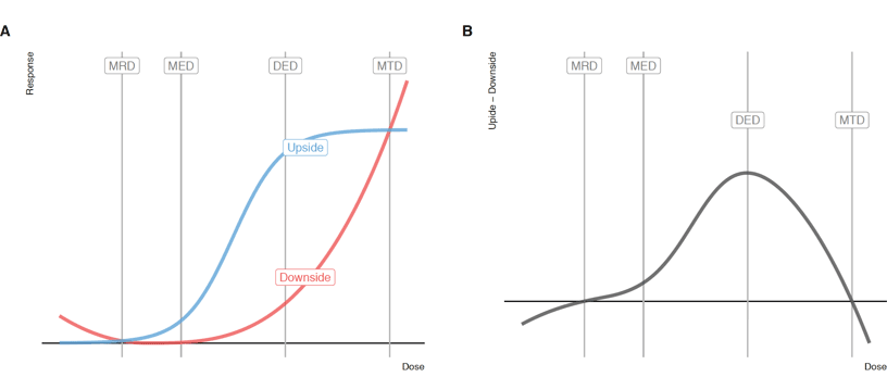
Figure 5.13. Hypothetical relationship between upside and downside. Panel A contains upside and downside as a separate curve, while panel B contains their difference. Vertical lines indicated different dose thresholds (see text for explanation)

Figure 5.13 depicts upside as the “S” shaped curve (i.e., sigmoid curve). Below MRD there is no upside, and after Diminishing Effect Dose (DED) threshold, increasing dose doesn’t increase the upside. MTD is the point where downsides overpower the upsides. DED also represent biggest difference (or ratio) between upside and downside (e.g. biggest bang for the buck).

Downside curve is represented as a parabolic curve. Below MRD, downside increases (i.e., detraining) and after MED downside curve exponentially rises, overcoming upside curve at MTD.

Please note that this is conceptual sandbox “Small World” model, and these thresholds are hard to pinpoint and are also dynamic (i.e., they change in time). Also, since this is a “Small World” model, there are also different approaches in differentiating the dose continuum. For example, Mike Israetel (Israetel, 2017) and the guys from Juggernaut Training Systems also utilize the following thresholds and zones: (1) Maintenance Volume (MV), (2) Minimum Effective Volume (MEV), (3) Maximum Adaptive Volume (MAV), (4) Maximum Recoverable Volume (MRV). MV is related to MRD, MEV is equal to MED, MAV is equal to DED (although this can be defined as a point where plateau starts, or where there is the biggest difference between upside and downside), MRV is equal to MTD.

Figure 5.14 contains visual depiction of MRD, MED, DED and MTD, as well as recovery, retention and development zone.

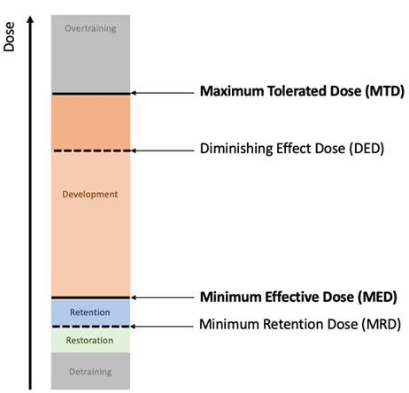
Figure 5.14. Position of the restoration, retention and development zones on the dose continuum between MED and MTD, with addition of MRD and DED thresholds

It is important to repeat one more time that these are theoretical constructs and this represents a “Small World” model. As demonstrated in the previous section of this chapter, a dose is tricky to define (e.g., over what time frame we define the dose? One session, one day, one week?), and even if we could, we would not be able to rely on the stationarity of the thresholds. It is thus interesting conceptual model.

3F Model: Fitness, Fatigue and Facilitation

Upside and Downside are easy components that are easy to grasp as two different qualitative types of adaptive response (positive and negative training effects). There are of course other models, for example Banister model (Clarke & Skiba, 2013) that involves two response components: (1) Fitness, and (2) Fatigue, which can be considered positive and negative training effects as well. I have expanded this model by adding third component facilitation or priming and I have called it the 3F model (see Figure 5.15). Each of these components of the response have a gain parameter and decay parameter (Clarke & Skiba, 2013). Without going into mathematical modeling, in simple terms, fitness is the upside which has medium gain, but slow decay (metastable level of performance or adaptation response). Fatigue is an example of the downside, that has highest gain (negative), but fast decay. Facilitation has small gain and fast decay, and in 3F model represents a component of the upside together with fitness. The idea of facilitation component is that sometimes athletes response to a “priming” session before a competition to “wake them up” and “prime” them for the competition. This effect can be psychological (e.g., confidence), but hey – it is still effect. Similar, but shorter time effect is PAP, or post activation potentiation. For example, PAP can be produced when one squats heavy (e.g., 85-90% 1RM for 1 rep or two) and after a short break achieves higher jump height than without performing the heavy squat in the first place.

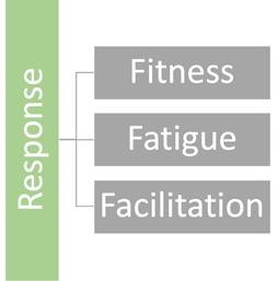
Figure 5.15. 3F model of response

The point behind 3F and Banister model, is that each dose creates fitness, fatigue and facilitation effects, and depending on the dose magnitude and sequencing, these three can play out differently across time. It is beyond the scope of this manual to go into Bannister or 3F mathematical modeling, but for the interested readers I highly recommend checking Clarke and  Skiba paper (Clarke & Skiba, 2013). This type of modeling (i.e., data informed, rather than data driven) can be useful in the Review and Retrospective phase (see Chapter 6), where one can collect a bunch of dose variables and use embedded testing, such as estimated 1RM from submax sets using velocity measurement, using estimated 1RM calculated using submit sets and subjective RIR ratings and so forth. This topic will be discussed in the Chapter 6 in much more detail.

Circular model

For the sake of example and simplicity, imagine that NL represents a training dose. Let’s say that the following weekly NL represents the aforementioned thresholds (see Table 5.8)

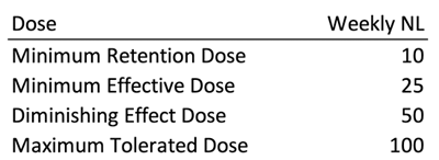
Table 5.8. Hypothetical scenario assuming weekly NL represents dose

Sounds scientific, right? Bollocks. Besides the obvious stupid assumption that NL represent dose (e.g., 25 weekly reps at what intensity? exercise?), consider the following. Imagine DED, which is equal to 50 NL in a week, is performed in one day, as opposed to five days. Will the response be the same? Will it be the same response if I am on a diet and my glycogen storage is low? If I had exams coming and I study the whole night, don’t get much sleep? My newborn kid is waking me 456 times a night? If I rate the workouts and sets as highly displeasurable?

Just thinking about this, it is immediately obvious that dose doesn’t have a direct causal link to response, but there is a moderator in between them: current state.

Figure 5.16 contains my circular “Small World” model of the dose -> response. Let me walk you through it.

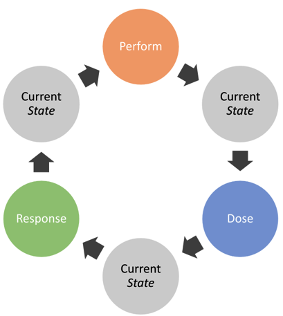
Figure 5.16. Circular causal pathway between performance, dose, response and current state

First of all, to create a dose (or adaptive stimuli), one needs to perform. If your current state is bad, you will not be able to perform, and thus the dose will be affected. As one performs, the amount and quality of stress (dose) created will also be moderated by the current state. Also, current state will be affected by the performance itself (e.g., performing better or worse than expected), dose and response. Depending on this very current state, adaptive response will be moderated. Pretty much everything affects everything. Besides, it might be hard to put a line between these components (e.g., is predicted 1RM using load-velocity relationship with warm-up sets a ‘response’ or ‘current state’?).

Current state is also a complex construct that is often reduced to the following quadrant (similar to dose quadrant on Figure 5.7).

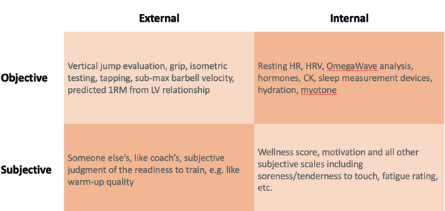
Figure 5.17. Current state quadrant

Current state can be thought of as two components: readiness and dose receptiveness. Readiness is related to the current ability to perform (e.g., due to sore legs, one is unable to perform heavy deep squats planned for today). Receptiveness is more complex and assumes that if equal dose is done in a better state (i.e., higher receptiveness state), higher response adaptation will be achieved (e.g., if you perform 5×5 with 150kg of heavy deep squats when your legs are fresh versus when they are tired, responses will be different). As always, these are “Small World” models and the underlying causal network might be much more complex than this. For example, performing heavy deep squats when sore, might actually provide a stronger stimuli for adaptive response, but can also impose downsides, for example in a form of prolonged soreness and heavy legs, which can affect other qualities development negatively. Or it could be that when fatigued, one cannot achieve a given standard of quality and dosage needed to create adaptation stimuli and response.

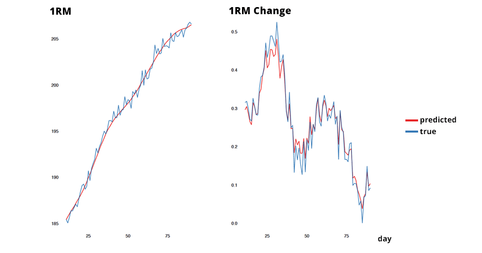
To assess a current state, the external in particular, one actually needs to perform. This means there is a blurry line between current state, performance, and response (adaptation). For example, to calculate estimated 1RM (either through 3-4 submit sets using LV profile, or using RIR) one needs to perform. The current adaptation level will also go inside estimated 1RM. The difference between response (or current level of adaptation) and current states is the time scale. Response is more long-term metastable level of performance (or trend, or adaptation response), while current state is more unstable and fluctuates. It can be said that performance equals sum of adaptation response and current state (see Figure 5.18), which is the same as 3F model, where response is the sum of fitness and fatigue (see Figure 5.15). For the sake of simplicity, we can assume that a current state can be considered as a sum of fatigue and facilitation from the 3F model. The following equation clarifies it: