Playing With Statistics [Part 4]
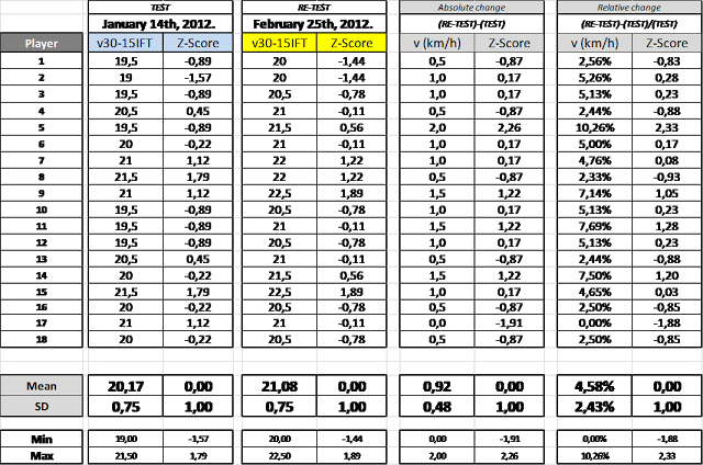
In the last part I did analysis of the test using standard score. Now I am going to analyze re-test. Here are the test score for both test and re-test.
| TEST | RE-TEST | |||||
|---|---|---|---|---|---|---|
| January 14th, 2012. | February 25th, 2012. | |||||
| Player | v30-15IFT | Z-Score | v30-15IFT | Z-Score | ||
| 1 | 19,5 | -0,89 | 20 | -1,44 | ||
| 2 | 19 | -1,57 | 20 | -1,44 | ||
| 3 | 19,5 | -0,89 | 20,5 | -0,78 | ||
| 4 | 20,5 | 0,45 | 21 | -0,11 | ||
| 5 | 19,5 | -0,89 | 21,5 | 0,56 | ||
| 6 | 20 | -0,22 | 21 | -0,11 | ||
| 7 | 21 | 1,12 | 22 | 1,22 | ||
| 8 | 21,5 | 1,79 | 22 | 1,22 | ||
| 9 | 21 | 1,12 | 22,5 | 1,89 | ||
| 10 | 19,5 | -0,89 | 20,5 | -0,78 | ||
| 11 | 19,5 | -0,89 | 21 | -0,11 | ||
| 12 | 19,5 | -0,89 | 20,5 | -0,78 | ||
| 13 | 20,5 | 0,45 | 21 | -0,11 | ||
| 14 | 20 | -0,22 | 21,5 | 0,56 | ||
| 15 | 21,5 | 1,79 | 22,5 | 1,89 | ||
| 16 | 20 | -0,22 | 20,5 | -0,78 | ||
| 17 | 21 | 1,12 | 21 | -0,11 | ||
| 18 | 20 | -0,22 | 20,5 | -0,78 | ||
| Mean | 20,17 | 0,00 | 21,08 | 0,00 | ||
| SD | 0,75 | 1,00 | 0,75 | 1,00 | ||
| Min | 19,00 | -1,57 | 20,00 | -1,44 | ||
| Max | 21,50 | 1,79 | 22,50 | 1,89 | ||
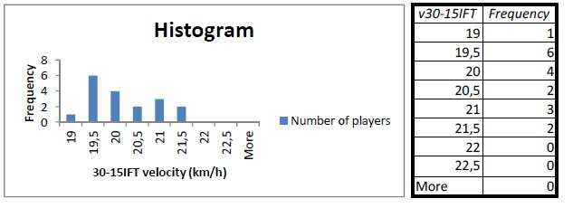
Here is the histogram of the two tests.
Now, there are two methods to calculate change (or improvement) between test and re-test IMHO. One is absolute where one just does the (re-test)-(test) (e.g. 21km/h – 19.5km/h, which is 1.5km/h) or relative which is this difference divided by the test [(re-test)-(test)]/(test) and that could be expressed as percentage (e.g. (21km/h – 19.5 km/h)/19.5, which is 7.69%. Honestly I don’t know which one is better, so I will utilize both. In the next table there is absolute change and relative change and their z-scores.
We see that the team improved for 4,58% on average (relative change) or for 0,92 km/h on average (absolute change).
The next thing I did is to create correlation table between these 4 data sets (test, re-test, absolute change, relative change).
| r | Test | Re-test | Absolute | Relative |
|---|---|---|---|---|
| Test | 1 | |||
| Re-test | 0,80 | 1 | ||
| Absolute | -0,31 | 0,33 | 1 | |
| Relative | -0,37 | 0,27 | 0,997 | 1 |
At the moment I don’t know how to measure significance and/or Student T test to test hypothesis, so I will only use Pearson’s correlation coefficient. (Someone please correct me if the thing I just said is plain gibberish)
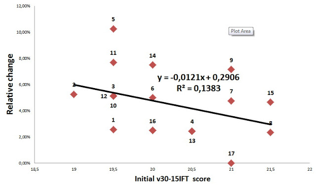
As we can see test and re-test have strong correlation (0,8) as well as relative and absolute change (0,997). We can also see the negative correlation between test and relative and absolute change (-0,31 and -0,37) which basically means that someone with higher test result will tend to show lower change. This is a common occurrence with almost all qualities – the more advanced you are the less (and harder) you improve over time. The correlation in this case is moderate (-0,37).
Here is the scatter of test and relative scores with the trend line.
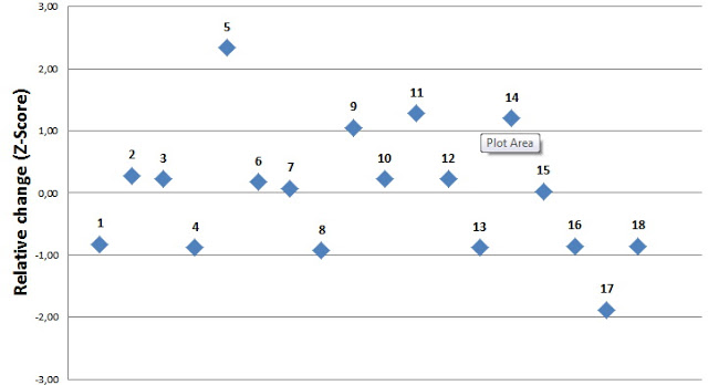
What is also interesting to do is to calculate the Z-score of the changes, which I did in the table. Using this we can identify outliers – those who are non-responders and those who are maybe on some form of AAS. Kidding aside, this is a useful tool.
From the graph above we can see that athlete number 5 improved for 10,26% with Z-score of 2,33. In this example he should be red flagged. This doesn’t mean anything, but rather necessities for more analysis. Maybe he did not push on the first test. Maybe there is an error in measurement. Maybe he took Ephedrine. Same with the guy number 17. He didn’t improve at all. He should be red flagged as well. Maybe he did not push in the re-test. Maybe he is non responder. Maybe the training was not enough for him (undertrained) or even too much (under-recovered), so he didn’t show any improvement. Basically, we don’t know thus he is a suspect for further analysis.
If you are more interested about responders and non-responder make sure to check this article and this one, and make sure to check mentioned papers within them (like Vollard et al., and Timmons et al.).
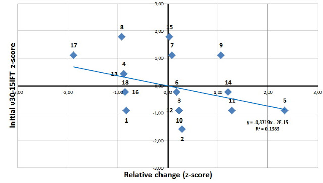
Going back to my four quadrant analysis – here is how the data looks with these athletes:
To be honest I got this idea WHILE I was writing this blog posts. This is why I actually like writing and reflecting – I got more ideas or they somehow emerge along the way. Anyway, I think that this idea of quadrants is very interesting. I can red-flag players and I can create different workouts based on their trainability and level of the certain tested quality. We can also identify potential talents, or non-responders. This might be interesting (especially if it could be applied to skills as well, like on the ball skills and decision making in the game) to identify strengths~weaknesses of the players and put them at certain playing positions (if they are non-responders) or modify training to get them more fit for different positions suited to coach style of play. IMHO it is interesting tool.
For example in the quadrant analysis above athletes 9 (higher initial score, higher responsiveness) and 1 (lower initial score, lower responsiveness) would probably demand different approach to training. It is beyond the scope of this article to go into how to utilize this quadrant analysis. It is also beyond my current knowledge as well – I am just starting to experiment with it.
That is for now folks. In the next installment I will cover how to do analysis for more frequent tests like sRPE, HRV and others we use for monitoring (this deals with comparing players baseline and his variability to himself rather than team average and variability). Stay tuned…





Responses