Optimal Force-Velocity Profile for Sprinting: Is It All Bollocks? – Part 5

In this installment I will do a simple simulation to acquire insights about the practical usefulness of the AVP and FVP optimization models. To achieve this, I will simulate large number of true sprint profile, with MSS ranging from 6 to 11 $ms^{-1}$, TAU ranging from 0.9 to 1.1 $s$ (since this is the most common range from the practice and published literature – (Clark and Ryan 2022; Samozino et al. 2022)), body height ranging from 155 to 195 $cm$, and body-mass-index (BMI) ranging from 18 to 25. BMI and body weight are used to calculate body weight, which ranged from 43 to 95 $kg$. These simulated parameters yielded 10,000 simulated sprint profiles.

Once we have these sprint profiles, we calculate the profile imbalance ($Profile_{IMB}$) using probing and slope method for AVP and FVP. The code below is used to generate this simulated data. Please note that it will take few hours to run. FVP Slope method utilized the max approach (which keeps the $P_{max}$ the same, as explained in the previous installment and Samozino et al. (2022)). The peak approach was not utilized in this simulation since it will take too long time to run.

require(shorts)
require(tidyverse)
require(kableExtra)
require(ggdist)
require(directlabels)

# ======================================
# Distribution of the profiles

# Simulation parameters
sim_params <- expand_grid(
  MSS = seq(6, 11, length.out = 10),
  TAU = seq(0.9, 1.1, length.out = 10),
  BH = seq(1.55, 1.95, length.out = 10),
  BMI = seq(18, 25, length.out = 10)
) %>%
  mutate(
    MAC = MSS / TAU,
    BW = round(BMI * BH^2, 0),
    BH = round(BH, 2),
    ID = row_number()
  ) %>%
  select(-BMI) %>%
  relocate(ID, MSS, MAC, TAU, BW, BH)

# FV Profile
fv_profile <- sim_params %>%
  rowwise() %>%
  mutate(as.data.frame(make_FV_profile(MSS, MAC, bodymass = BW, bodyheight = BH)[c("F0_poly", "V0_poly")])) %>%
  ungroup() %>%
  rename(F0 = F0_poly, V0 = V0_poly)


# Profile imbalance
profile_imb <- fv_profile %>%
  expand_grid(dist = seq(1, 30, by = 1)) %>%
  mutate(
    `AVP Probe` = probe_MSS_MAC(dist, MSS, MAC)$profile_imb,
    `AVP Slope` = optimal_MSS_MAC(dist, MSS, MAC)$profile_imb,
    `FVP Probe` = probe_FV(dist, F0, V0, bodymass = BW, bodyheight = BH)$profile_imb,
    `FVP Slope` = optimal_FV(dist, F0, V0, bodymass = BW, bodyheight = BH)$profile_imb
  )

# Convert to long
profile_imb_long <- profile_imb  %>%
  pivot_longer(
    cols = c(`AVP Probe`, `AVP Slope`, `FVP Probe`, `FVP Slope`), 
    names_to = "method")

# Distribution of profiles
profile_imb_perc_deficit <- profile_imb_long %>%
  group_by(method, dist) %>%
  summarise(
    `% Velocity deficit` = 100 * sum(value > 105) / n(),
    `% Force deficit` = 100 * sum(value < 95) / n()
  ) %>%
  ungroup() %>%
  pivot_longer(cols = c(`% Velocity deficit`, `% Force deficit`), names_to = "deficit")

Figure 1 depicts results of this simulation. Black line represents the median $Profile_{IMB}$ across simulated profiles, while the shaded aread represents the 99% of the distribution.

significance <- 0.99

profile_imb_long %>%
  ggplot(aes(x = dist, y = value)) +
  theme_linedraw(8) +
  stat_lineribbon(.width = significance, size = 0.5, alpha = 0.9) +
  scale_fill_brewer(palette = "Blues") +
  geom_hline(yintercept = 100, linetype = "dotted") +
  facet_wrap(~method) +
  xlab("Distance (m)") +
  ylab("Profile Imbalance (%)") +
  theme(legend.position = "none")

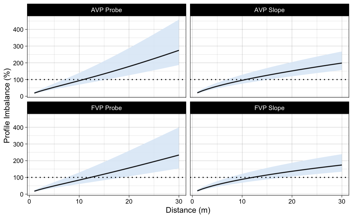
Figure 1: Median and 99% distribution interval of the Profile Imbalance metric using simulated data

Figure 2 depicts the simulation results for the FVP Slope method only, since that is the method utilized in Samozino et al. (2022).

fv_slope_profile_imb <- profile_imb_long %>%
  filter(method == "FVP Slope")

# Find crossings
df <- fv_slope_profile_imb %>%
  group_by(dist) %>%
  summarise(
    median = median(value),
    lower = quantile(value, 1 - (significance +  (1 - significance)/2)),
    upper = quantile(value, (significance +  (1 - significance)/2))
  )

m_median <- lm(median~poly(dist, 3), df)
m_lower <- lm(lower~poly(dist, 3), df)
m_upper <- lm(upper~poly(dist, 3), df)

cross_100 <- function(dist, model) {
  100 - predict(model, data.frame(dist = dist))
}

median_dist <- uniroot(cross_100, lower = 1, upper = 50, model = m_median)$root
lower_dist <- uniroot(cross_100, lower = 1, upper = 50, model = m_lower)$root
upper_dist <- uniroot(cross_100, lower = 1, upper = 50, model = m_upper)$root

# Plot
fv_slope_profile_imb %>%
  ggplot(aes(x = dist, y = value)) +
  theme_linedraw(8) +
  stat_lineribbon(.width = significance, size = 0.5, alpha = 0.9) +
  scale_fill_brewer(palette = "Blues") +
  geom_hline(yintercept = 100, linetype = "dotted") +
  geom_vline(xintercept = c(lower_dist, upper_dist), linetype = "dotted") +
  annotate("text", x = upper_dist, y = 30, label = paste(" ", round(upper_dist, 1)), hjust = "left") +
  annotate("text", x = lower_dist, y = 30, label = paste(round(lower_dist, 1), " "), hjust = "right") +
  xlab("Distance (m)") +
  ylab("Profile Imbalance (%)") +
  theme(legend.position = "none")

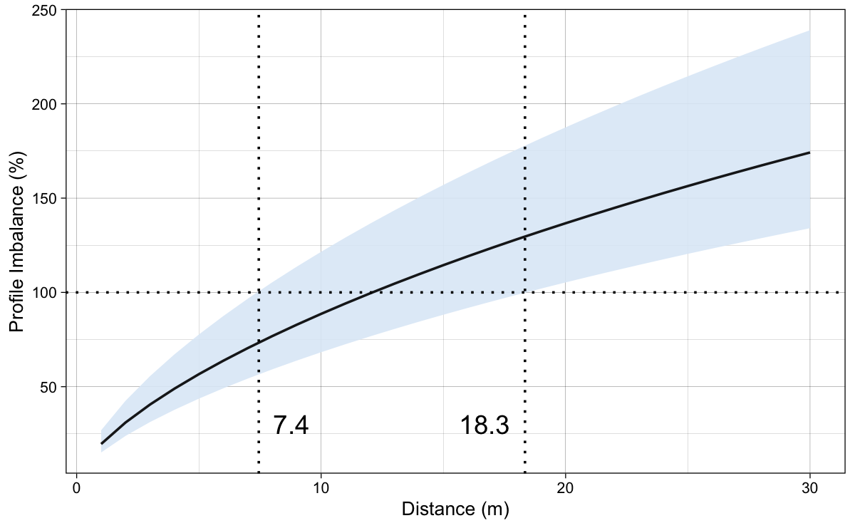
Figure 2: Median and 99% distribution interval of the Profile Imbalance metric using simulated data for the FVP Slope method

What can we conclude from Figure 2 in this simulation analysis? In plain English, FVP optimization is pretty much useless for the distances shorter that 7.4$m$ and longer than 18.3$m$ since all simulated profiles are “Force Deficient” and “Velocity Deficient” respectively. No shit braniac! Tell me something we didn’t know.

I am not against using the FVP optimization analysis, but please do not make it as something magical and scientific. We have shown the assumptions of this model and the potential problem (i.e., $P_{peak}$ not being the same as the slope changes), as well as the the results of this simple simulation aligning the FVP optimization results with simple and already know heuristic: “To improve your sub 10m split times, work on acceleration traits by doing shorter sprints. To improve your over 20m split times, work on your max speed traits by doing longer sprints” (WARNING: here we also assumed independence of these traits, as well as assuming that there are clear methods (e.g., long vs short sprints) to directly target these traits, but the collective wisdom of sprint coaches across time is not something to simply disregard as Is~Ought Gap).

All is all, optimal FVP is bollocks – please do not waste tax payers money in researching “whether training based on your optimal FV sprint profile yields better improvements in split times”. Roasting of the Samozino et al. (2022) is done, I am out.

References

1. Clark, Kenneth P., and Laurence J. Ryan. 2022. “Hip Torque Is a Mechanistic Link Between Sprint Acceleration and Maximum Velocity Performance: A Theoretical Perspective.” Frontiers in Sports and Active Living 4 (July): 945688. https://doi.org/10.3389/fspor.2022.945688.
2. Samozino, Pierre, Nicolas Peyrot, Pascal Edouard, Ryu Nagahara, Pedro Jimenez-Reyes, Benedicte Vanwanseele, and Jean-Benoit Morin. 2022. “Optimal Mechanical Force–Velocity Profile for Sprint Acceleration Performance.” Scandinavian Journal of Medicine & Science in Sports 32 (3): 559–75. https://doi.org/10.1111/sms.14097.