Banister Impulse~Response model in R [part 3]

Here is the another ‘playbook’, but this time on my own data set during high-frequency project I did in 2013. The data set features estimated 1RM using velocity (which I measure during the lifts). I have also measure Peak Velocity and Mean Power in CMJ w/20kg before lowerbody workouts. Those four are response variables.

The impulse variables are squat and bench press volume, tonnage, impulse (%1RM * reps * sets) and corrected impulse (using daily corrected %1RM based on daily 1RM).

library(lubridate)

# Load Banister functions
source("Banister Impulse Response Multivariate.R")

# Load data
mladen.data <- read.csv("Mladen-Analysis-High-Freq.csv", header = TRUE)
str(mladen.data)

## 'data.frame':    25 obs. of  13 variables:
##  $ Date                         : Factor w/ 25 levels "","1.5.13","10.4.13",..: 3 4 5 6 7 8 9 10 11 12 ...
##  $ Squat.est.1RM                : num  178 NA 191 NA 164 ...
##  $ Bench.est.1.RM               : num  NA 119 NA 119 NA ...
##  $ CMJ.PV                       : num  3.1 3.13 3.08 3.17 3.17 3.22 NA NA 3.13 3.13 ...
##  $ CMJ.MP                       : num  634 647 624 670 669 ...
##  $ Bench.Press.Volume           : int  NA 12 NA 24 NA 18 NA NA NA 10 ...
##  $ Bench.Press.Tonnage          : int  NA 1056 NA 1980 NA 1386 NA NA NA 935 ...
##  $ Bench.Press.Impulse          : num  NA 9.6 NA 18 NA 12.6 NA NA NA 8.5 ...
##  $ Bench.Press.Corrected.Impulse: num  NA 8.8 NA 16.7 NA 12 NA NA NA 8.1 ...
##  $ Squat.Volume                 : int  24 NA 18 NA 12 NA NA NA 21 NA ...
##  $ Squat.Tonnage                : int  2880 NA 2016 NA 1536 NA NA NA 2688 NA ...
##  $ Squat.Impulse                : num  18 NA 12.6 NA 9.6 NA NA NA 16.8 NA ...
##  $ Squat.Corrected.Impulse      : num  16.1 NA 10.6 NA 9.3 NA NA NA 19.4 NA ...

But before we model using the Banister function, we need to get rid of NAs in the impulse columns, which in this case represent zero. We also need to fix the dates in the first column.

mladen.data$Date <- dmy(mladen.data$Date) 

impulse.columns <- mladen.data[6:13]
impulse.columns[is.na(impulse.columns)] <- 0

mladen.data <- cbind(mladen.data[1:5], impulse.columns)

Let’s create a model for bench press (est 1RM).

# Create multiple models for estimated bench press using different impulse metrics

bench.model1 <- train.Banister(data=mladen.data,
                               impulse="Bench.Press.Volume",
                               response="Bench.est.1.RM")

bench.model2 <- train.Banister(data=mladen.data,
                               impulse="Bench.Press.Tonnage",
                               response="Bench.est.1.RM")

bench.model3 <- train.Banister(data=mladen.data,
                               impulse="Bench.Press.Impulse",
                               response="Bench.est.1.RM")

bench.model4 <- train.Banister(data=mladen.data,
                               impulse="Bench.Press.Corrected.Impulse",
                               response="Bench.est.1.RM")

# plot all four models
plot.banister(bench.model1)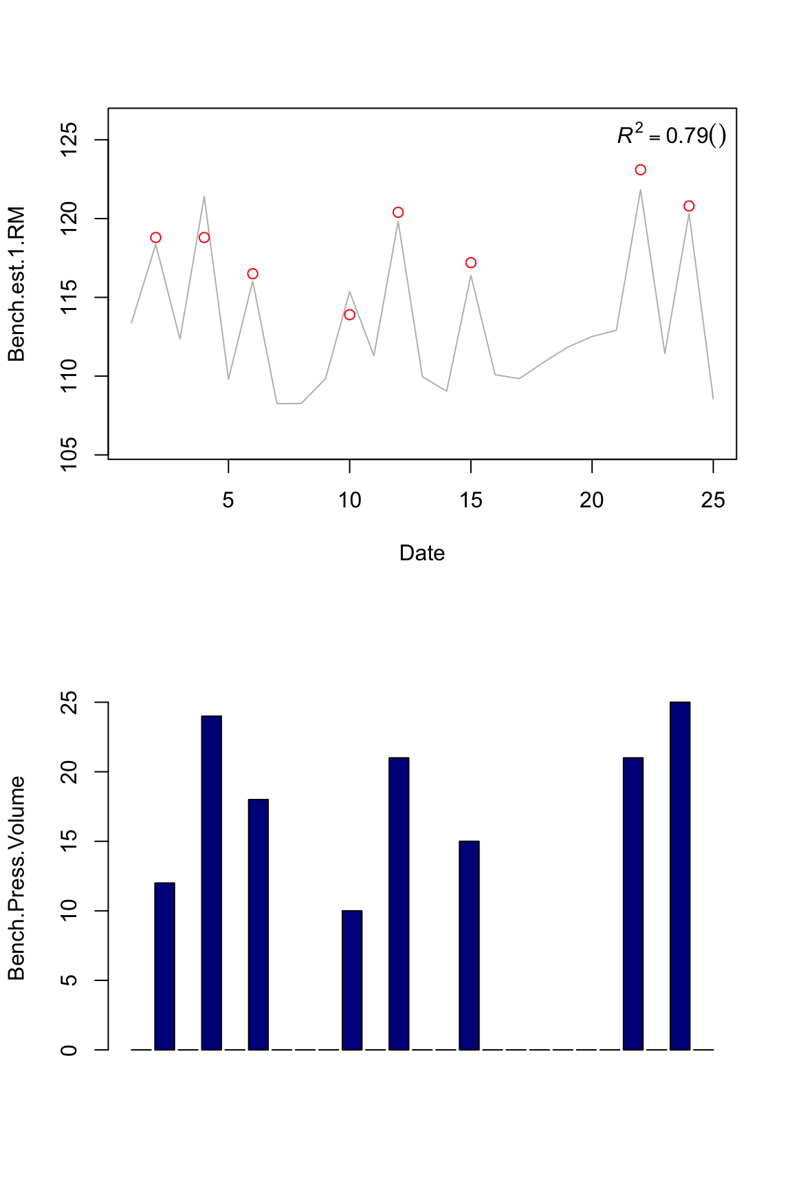

plot.banister(bench.model2)

plot.banister(bench.model3)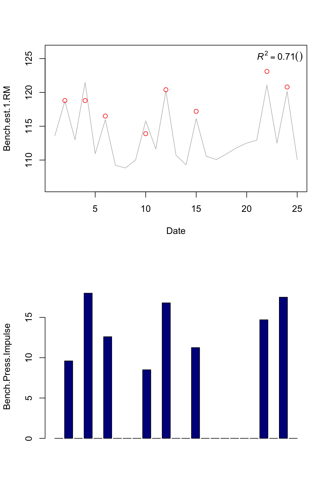

plot.banister(bench.model4)

Now the question is which impulse metric is the best predictor? Using machine learnin terminology, since this is a “training” set, a model that has high R squared might not have high R squared in a “testing” set. So we don’t know if our model is overfitting (please see recommended literature on machine learning ).

Another important issues is garbage in, garbage out. We can’t just feed out model with everything – we need to invest some time and energy to find the best predictor or combination of predictors (that also don’t overfit). For example, all these measure correlate so there is no much point in including all of the in the model. All these measure don’t catch all information regarding training: for example, I can ramp up tonnage by doing a lot of reps and sets with very low %1RM, as I can do with higher %1RM.

There is more art than science in model building for sure.

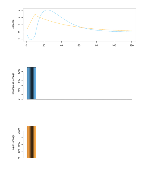
So for this exmple I will use volume parameter since it has the higher “training” R squared. Let’s see how our model looks like for both squat and bench press 1RM using squat and bench tonnage.

model1 <- train.Banister(data=mladen.data,
                               impulse=c("Bench.Press.Tonnage", "Squat.Tonnage"),
                               response=c("Bench.est.1.RM", "Squat.est.1RM"))

plot.banister(model1)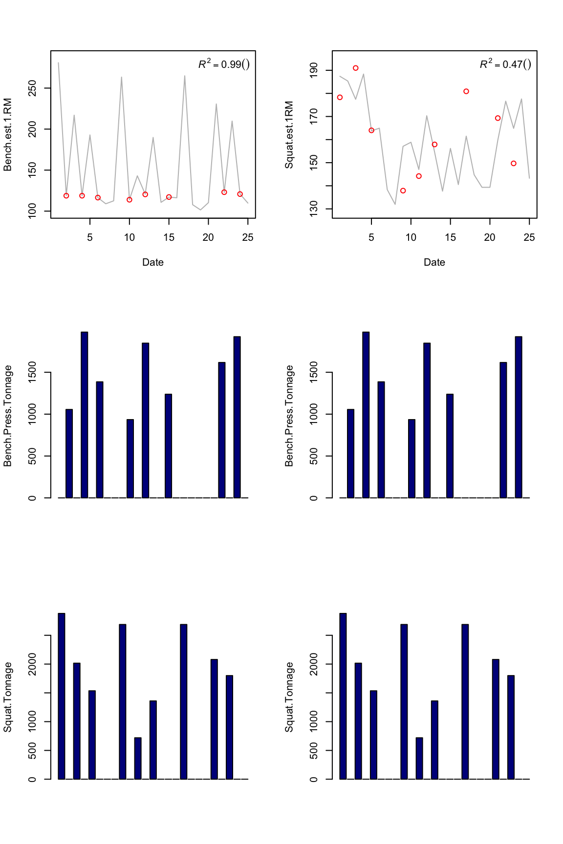

As you can see from the picture for the bench press, even if we got perfect R squared, the predicted values swing to 250kg. I can’t press 140kg – I can only dream of 250. So R squared might not be a best marker for the fit and we need to check the graph.

Let’s see the squat 1RM if we use different metrics

squat.model1 <- train.Banister(data=mladen.data,
                               impulse="Squat.Volume",
                               response="Squat.est.1RM")

squat.model2 <- train.Banister(data=mladen.data,
                               impulse="Squat.Tonnage",
                               response="Squat.est.1RM")

squat.model3 <- train.Banister(data=mladen.data,
                               impulse="Squat.Impulse",
                               response="Squat.est.1RM")

squat.model4 <- train.Banister(data=mladen.data,
                               impulse="Squat.Corrected.Impulse",
                               response="Squat.est.1RM")

plot.banister(squat.model1)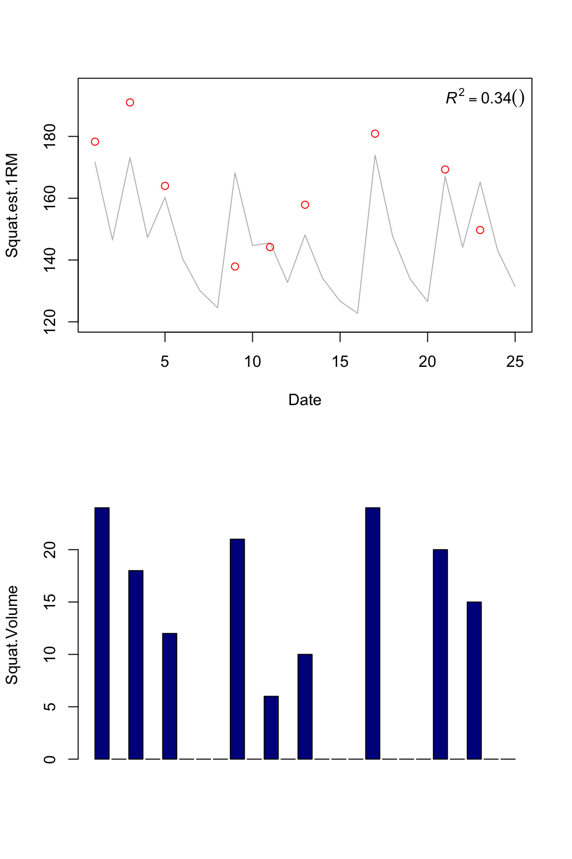

plot.banister(squat.model4)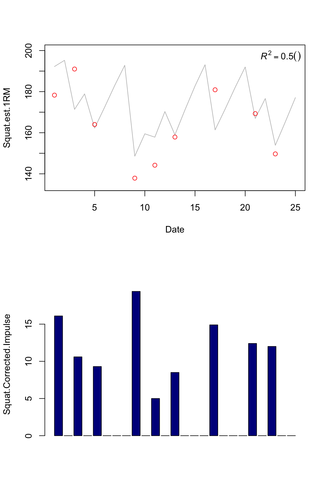

We can see that different metrics have different R squared. This might mean that they are garbage and can’t predict much. Hence we get garbage out.

What we can do with a larger sample of data is to crossvalidate or basically split the data in “training” and “testing” – which means we learn/train our models on “training data” and evaluate their precision on “testing data”. We can try different combos of impulse metrics available and see which one can give us the best prediction without overfitting.