Optimal Force-Velocity Profile for Sprinting: Is It All Bollocks? – Part 1

In this article series I will provide my opinion regarding the use of Force-Velocity Profile (FVP) optimization for short sprints (i.e., the sprints where there is no deceleration). Recent paper by Pierre Samozino et al. (2022) continues this FVP optimization theme from jumping [Pierre Samozino et al. (2012); Pierre Samozino (2018); P. Samozino et al. (2013); Pierre Samozino et al. (2008)]¹, but now applied to short sprinting. Before I offer my opinion, I will need to walk you through the whole process.

In this article series I will use the {shorts} package (Jovanović and Vescovi 2022; Jovanović 2022) for R programming language (R Core Team 2022). Code will be provided, but for more thorough introductions, please check the provided references.

Sprint models

There are multiple ways of how sprint models are created (e.g., using timing gates, video analysis, radar/laser guns, tether devices), but in first part of this article series, I will use the radar/laser gun. With radar/laser gun method, athlete accelerates maximally until reaching top speed (it depends on the level/sport, but 40m for your average team sport athlete is usually enough). Radar or laser gun is pointed to the athlete upper or lower back, and the captured velocity is assumed to be center-of-mass (COM) velocity. Frequency of capturing this velocity is often pretty high (e.g., 100Hz or more; in other words 100 samples in a second).

There are some issues with collecting this velocity when athletes start from the crouch position instead of the standing start, but I will disregard them for the purpose of this article. Figure 1 depicts one such sprint. Please notice that the grey line, which represents the raw or instantaneous velocity, fluctuates. This is due to deccelerations and re-accelerations from step to step. There is certainly some noise involved (which can make havoc when estimating acceleration or the 1st derivative), but we will disregard it here. To provide average step velocity, the radar or laser software also provides some smoothed velocity (see black line on Figure 1). This is achieved by using certain filters (i.e., Kalman for example). And this is where we make our first model approximation (actually second, if we disregarding the assumption that low/upper back velocity is COM velocity). This assumption is that the COM velocity is smooth (by averaging step velocities, so to speak).

require(tidyverse)
require(shorts)
require(cowplot)
require(directlabels)

# Prepare data
laser_df <- read_csv("data/sample-laser.csv") %>%
  mutate(Time = Time / 1000)

# Get the deceleration location with simple heuristic
dec_time <- laser_df$Time[which.max(laser_df$Smooth)]

# Plot
ggplot(laser_df, aes(x = Time, y = `Raw-Velocity`)) +
  theme_linedraw(8) +
  annotate(
    "rect",
    xmin = dec_time, xmax = 5.5, ymin = 6.5, ymax = 7.5,
    fill = "grey", alpha = 0.5
  ) +
  annotate(
    "text",
    x = dec_time, y = 7.6, hjust = "left", vjust = "bottom",
    label = "Decceleration", size = 2.5
  ) +
  geom_line(alpha = 0.8, color = "grey") +
  geom_line(aes(y = Smooth), alpha = 0.8, color = "black") +
  scale_color_brewer(palette = "Set1") +
  xlab("Time (sec)") +
  ylab("Velocity (m/s)")

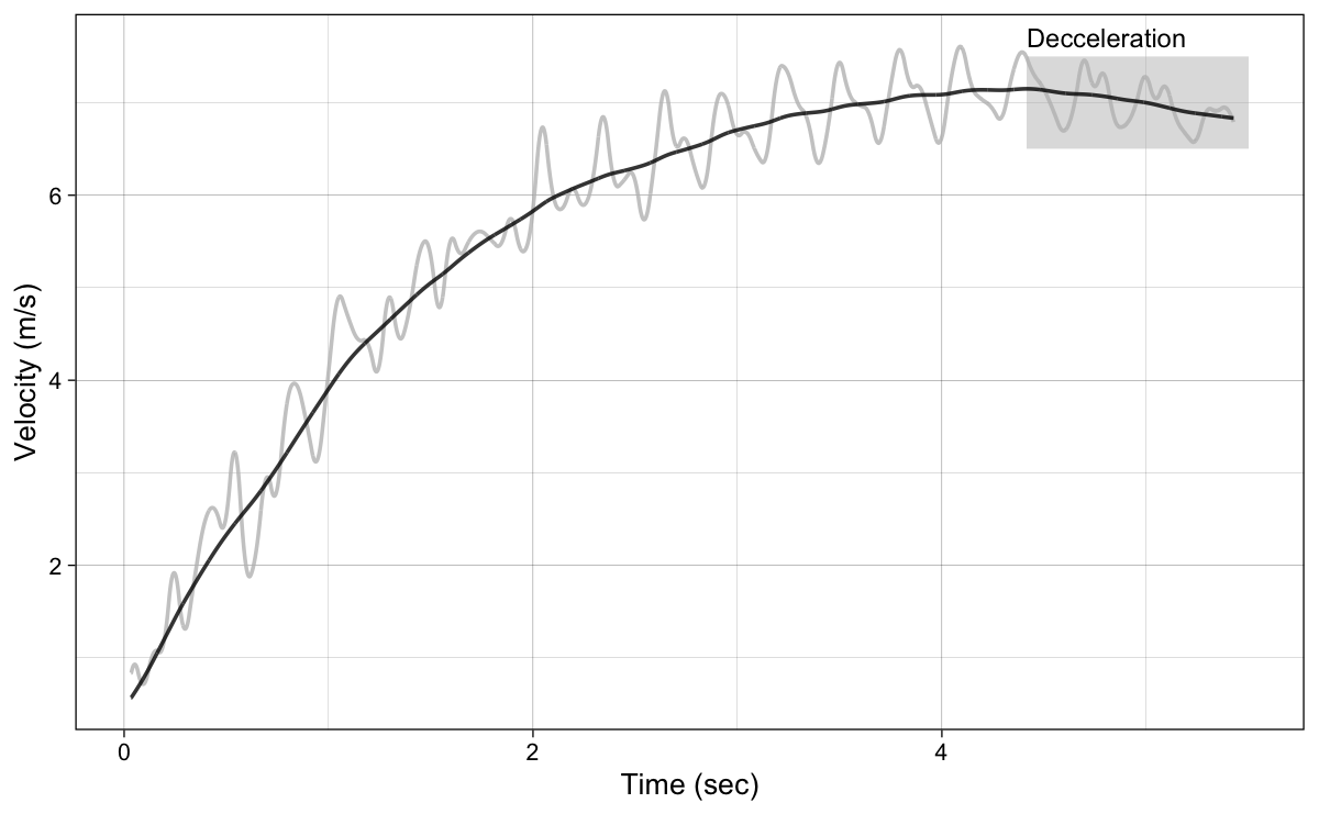
Figure 1: Short sprint velocity using radar/laser gun. Notice the fluctuations in raw/ instantaneous velocity (grey line), which is due step-to-step decceleration/acceleration. Black line represents smoothed velocity using certain types of filter, to yield aproximate average step velocity. Grey area is where athlete starts to deccelerate, and this phase should be filtered out from our sample

It is important to keep in mind that the models are simplifications of the reality, built to describe, predict, and sometimes explain and intervene on phenomena we regularly observe. In other words, we try to create a simplified map of the Large World using Small World models (McElreath 2020; Savage 1972; Binmore 2011; Volz and Gigerenzer 2012; Gigerenzer, Hertwig, and Pachur 2015; Jovanović 2020). These are always wrong, but can be useful, sometime they can even be harmful (i.e., when making erroneous intervention claims, by assuming causal explanation of the model). I will come back to this dichotomy thorough this article series.

Instead of using simple filtering to smooth out the sprint velocity, we can fit (1) 3rd degree polynomial model (Equation 1), and (2) mono-exponential model (Equation 2) (implemented in the {shorts} package). I will explore these two, but we will use mono-exponential model as a gold standard to model velocity performance during short sprints. In the second part of this article series I will focus solely on the mono-exponential model and its characteristics.

\begin{split}v(t) = b_0 + b_1 \times t + b_2 \times t^2 + b_3 \times t^3 \\\end{split}

Equation 1

\begin{split}v(t) = MSS \times (1 – e^{-\frac{t}{TAU}}) \\\end{split}

Equation 2

Before we continue with our modeling aims, we need to filter-out that grey deceleration phase from Figure 1. The question is how do we decide at which point in time one start to deccelerate? This is additional subjective input in our modeling (the science-is-objective crowd will roll their eyes here). For the sake of this example, I will use peak smoothed velocity and remove everything after that.

Figure 2 depicts model predictions. In other words, these models (with the exception of the smooth model), map-out the relationship between time (i.e., predictor variable) and raw velocity (i.e., target or outcome variable).

# Remove deceleration section
laser_df <- laser_df %>%
  filter(Time <= dec_time)

# Make models

# Mono-exponential
m1 <- shorts::model_radar_gun(
  time = laser_df$Time,
  velocity = laser_df$`Raw-Velocity`
)

# Polynomial model
m2 <- lm(`Raw-Velocity` ~ poly(Time, 3), laser_df)

# Add prediction
laser_models_df <- laser_df %>%
  mutate(
    `Mono-exponential` = predict(m1),
    `Polynomial` = predict(m2)
  ) %>%
  # convert to long
  pivot_longer(cols = -Time, names_to = "model", values_to = "velocity") %>%
  mutate(model = factor(model, levels = c("Raw-Velocity", "Smooth", "Polynomial", "Mono-exponential"))) %>%
  # Get Acceleration and power
  group_by(model) %>%
  arrange(Time) %>%
  mutate(
    dv = c(NA, diff(velocity)),
    dt = c(NA, diff(Time)),
    acceleration = dv/dt,
    net_relative_power = velocity * acceleration
  ) %>%
  ungroup()


# Plot velocity
ggplot(
  laser_models_df %>% 
    filter(model != "Raw-Velocity"),
  aes(x = Time, y = velocity, color = model)) +
  theme_linedraw(8) +
  geom_line(
    data = laser_models_df %>% 
    filter(model == "Raw-Velocity"), 
    aes(x = Time, y = velocity),
    color = "grey",
    alpha = 0.8
  ) +
  geom_line(alpha = 0.8) +
  scale_color_brewer(palette = "Set1") +
  xlab("Time (sec)") +
  ylab("Velocity (m/s)") +
  theme(legend.position = "none") +
  geom_dl(
    aes(label = paste("  ", model)),
    method = list("last.bumpup", cex = 0.5)
  ) +
  xlim(0, 5.5) + 
  ylim(0, 9)

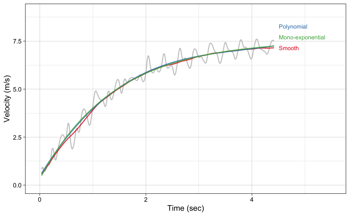
Figure 2: Short sprint velocity using radar/laser gun. To “smooth” out the fluctuations, multiple models could be used. Here we have depicted software smoother (most likely using some type of Kalman filter), as well as polynomial (3rd degree) and mono-exponential model predictions

As can be seen from Figure 2, polynomial and mono-exponential models provide almost identical model predictions or model fit (standard error of the estimate equal to 0.332 and 0.334 $ ms^-1$ respectively). Before I embark on the benefits of using mono-exponential model (which should be more evident as you read anyway), let’s explore other kinematic variables: acceleration and power.

To estimate acceleration, we need to do 1st derivative (i.e., how fast is the velocity changing). In other words, we need to divide the change in velocity (i.e., $ \Delta v $) with change in time ($ \Delta t $). We can do this (1) computationally, and (2) algebraically using the actual models themselves. Algebraic method involves solving some ordinary differential equations (ODE) for the polynomial model and mono-exponential model (which is easier to be done and can be found in Equation 3).

\begin{split}a(t) = \frac{MSS}{TAU} \times e^{-\frac{t}{TAU}}\\\end{split}

Equation 3

But to provide the fair treatment to raw and smoothed velocity, I will estimate and plot acceleration using computational method by dividing change in velocity (i.e., difference between two adjunct samples in the data) by the change in time (or more simply by the 1/sampling rate). Result of this method is plotted in Figure 3. Note that Figure 3 have two figures - Figure 3 (a) includes acceleration estimated using raw velocity (grey line), while Figure 3 (b) excludes it for a better view of the model estimated acceleration.

# Plot acceleration
ggplot(
  laser_models_df %>% 
    filter(model != "Raw-Velocity"),
  aes(x = Time, y = acceleration, color = model)) +
  theme_linedraw(8) +
  geom_hline(yintercept = 0, linetype = "dotted") +
  geom_line(
    data = laser_models_df %>% 
    filter(model == "Raw-Velocity"), 
    aes(x = Time, y = acceleration),
    color = "grey",
    alpha = 0.8
  ) +
  geom_line(alpha = 0.8) +
  scale_color_brewer(palette = "Set1") +
  xlab("Time (sec)") +
  ylab("Acceleration (m/s/s)") +
  theme(legend.position = "none") +
  geom_dl(
    aes(label = paste("  ", model)),
    method = list("last.bumpup", cex = 0.5)
  ) +
  xlim(0, 5.5)

ggplot(
  laser_models_df %>% 
    filter(model != "Raw-Velocity"),
  aes(x = Time, y = acceleration, color = model)) +
  theme_linedraw(8) +
  geom_hline(yintercept = 0, linetype = "dotted") +
  geom_line(alpha = 0.8) +
  scale_color_brewer(palette = "Set1") +
  xlab("Time (sec)") +
  ylab("Acceleration (m/s/s)") +
  theme(legend.position = "none") +
  geom_dl(
    aes(label = paste("  ", model)),
    method = list("last.bumpup", cex = 0.5)
  ) +
  xlim(0, 5.5)

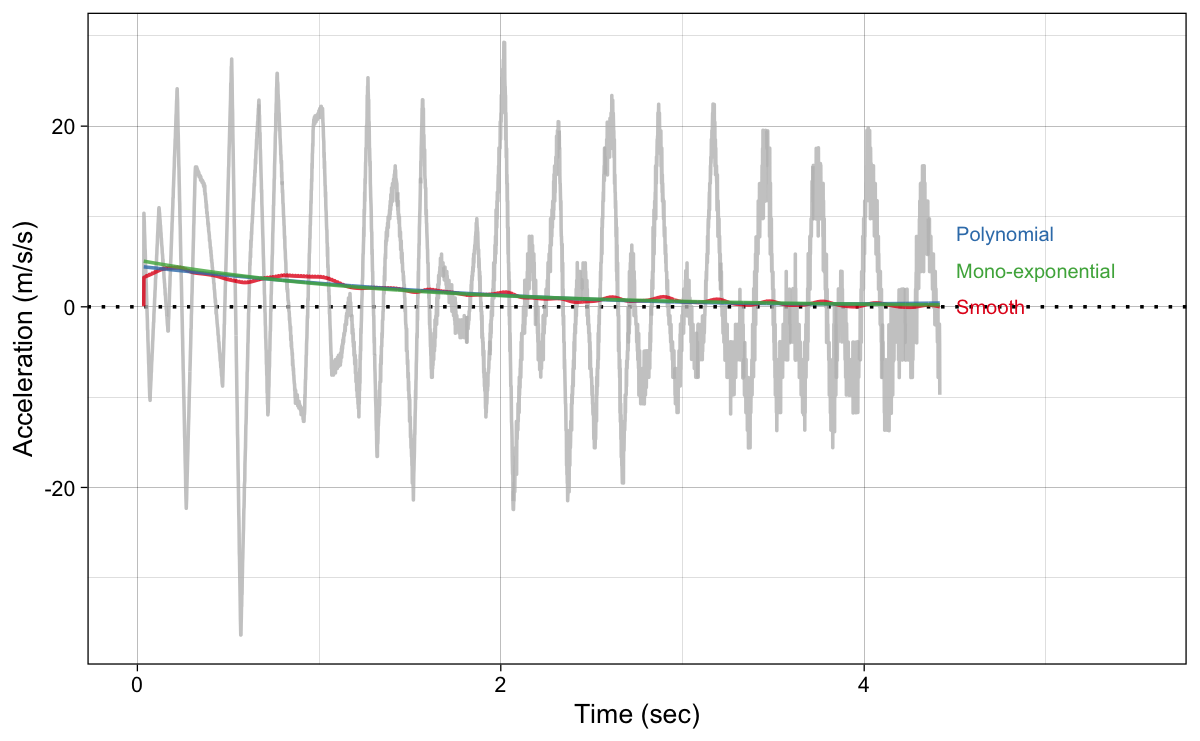
(a) Estimated acceleration using raw velocity

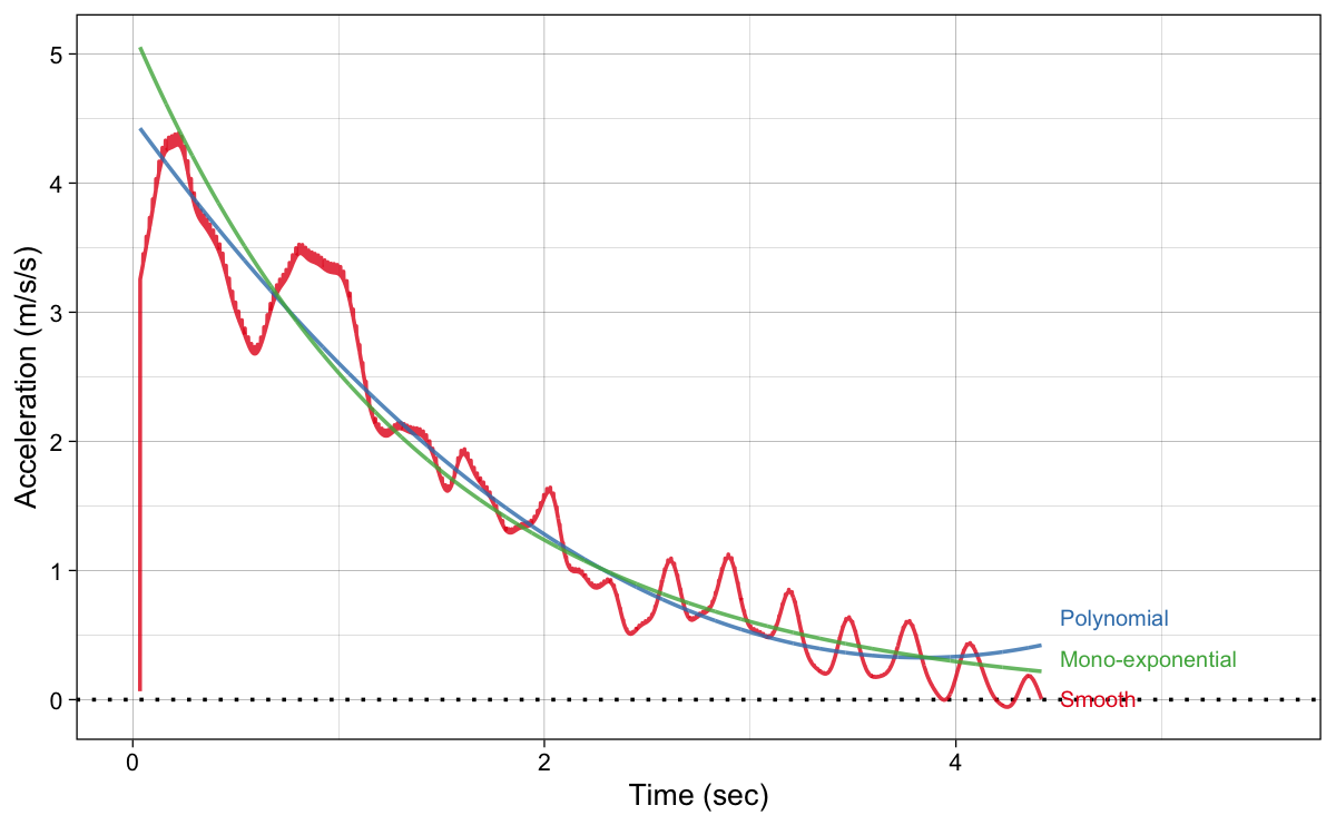
(b) Estimated acceleration using model predictions

Figure 3: Estimated acceleration using dt/dv

There are few things to notice from Figure 3. First, see how the estimated acceleration from the raw velocity is wild. This can be due to measurement noise that is included in the raw signal, which is magnified when doing the first derivative. But this can also be the real acceleration phenomena, where on each step there are acceleration and decceration cycles (which can also help us identify steps and maybe quantify left-right side differences or asymmetries, but this is a topic for another article). These magnitudes might also be telling a story that we can use - for example we might notice that someone might be breaking too much due to overstriding or what have you. Anyway, these should not be thrown out easily for the more gross (or smoothed out, or averaged out) accelerations we get from the models or model predictions.

Second thing to notice is the acceleration estimated from the smoothed velocity. This is also wild, but less than the acceleration estimated from the raw velocity values.

Third thing to notice is the difference between estimated acceleration using polynomial and mono-exponential velocity predictions. Mono-exponential model demonstrated higher initial acceleration (this is equal to $ MAC $; maximal acceleration or $ \frac{MSS}{TAU} $ which I will explain in more details in the next installment) that tapers down to zero. Contrary to this, polynomial model estimated acceleration is lower at the start, but it has this weird increase at the end of the sprint. This model is thus theoretically unsound (keep counting these drawbacks please).

Let’s estimate net relative power (in W/kg). To do this we just multiply velocity with estimated acceleration. Why is this called net power? Because, this is not the total power generated by the athlete, but only power involved in increasing the momentum or the kinetic energy. To estimate total power, we need to have other resisting forces (e.g., air resistance) and work done (e.g., accelerating and decelerating limbs, which can demand more that 80% energy generated - I do not have a reference for this, sorry evidence-based zealots. Must have been in the Bosch book somewhere). And why is it called relative? Because it is relative to bodyweight or mass of the athlete.

Estimated net relative power (in W/kg) is depicted in Figure 4.

# Plot net relative power
ggplot(
  laser_models_df %>% 
    filter(model != "Raw-Velocity"),
  aes(x = Time, y = net_relative_power, color = model)) +
  theme_linedraw(8) +
  geom_line(
    data = laser_models_df %>% 
    filter(model == "Raw-Velocity"), 
    aes(x = Time, y = net_relative_power),
    color = "grey",
    alpha = 0.8
  ) +
  geom_line(alpha = 0.8) +
  scale_color_brewer(palette = "Set1") +
  xlab("Time (sec)") +
  ylab("Net Relative Power (W/kg)") +
  theme(legend.position = "none") +
  geom_dl(
    aes(label = paste("  ", model)),
    method = list("last.bumpup", cex = 0.5)
  ) +
  xlim(0, 5.5)

ggplot(
  laser_models_df %>% 
    filter(model != "Raw-Velocity"),
  aes(x = Time, y = net_relative_power, color = model)) +
  theme_linedraw(8) +
  geom_line(alpha = 0.8) +
  scale_color_brewer(palette = "Set1") +
  xlab("Time (sec)") +
  ylab("Net Relative Power (W/kg)") +
  theme(legend.position = "none") +
  geom_dl(
    aes(label = paste("  ", model)),
    method = list("last.bumpup", cex = 0.5)
  ) +
  xlim(0, 5.5)

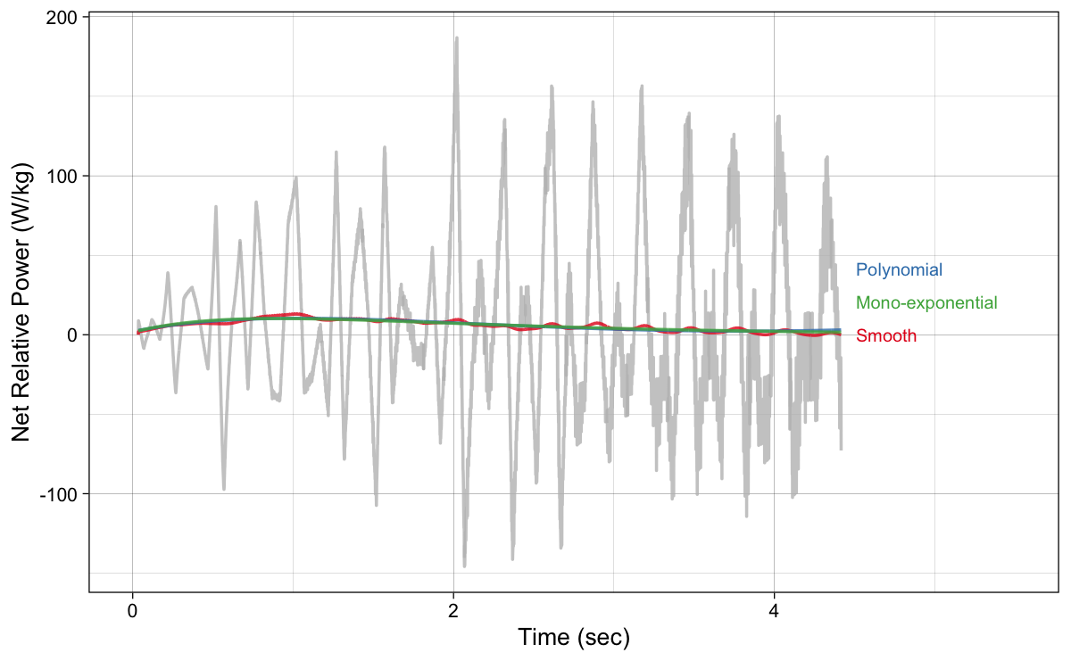
(a) Estimated power using raw velocity and raw acceleration

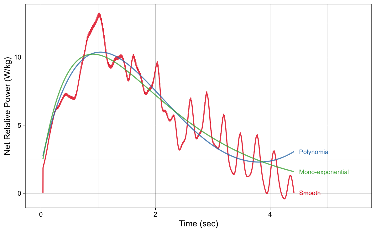
(b) Estimated power using model predicted velocity and acceleration

Figure 4: Estimated net relative power using acceleration x velocity

Similarly to acceleration, there are few thing to notice from Figure 4. Power estimated from raw velocity and acceleration is all over the place. Again, this could be due to measurement noise, or it could be the real phenomena due to step to step accelerations and deccelerations.

Power estimated using model predictions demonstrates asymmetrical bell-shape with a prominent peak value (this value is called $ P_{peak} $ and represent maximal net power manifested). For the mono-exponential model, this is equal to $ \frac{MSS \times MAC}{4} $, which is another simplicity (or mathematical elegance) benefit of the mono-exponential model. Notice that power estimated using mono-exponential model tapers of to zero (not shown in Figure 4), which is in alignment with our theoretical understanding (i.e., when reaching steady velocity, net power is equal to zero). This is not the case for the polynomial model.

Another interesting analysis is the relationship between acceleration and velocity, or Acceleration-Velocity Profile (AVP). This simply done by plotting each sampled velocity with estimated acceleration (Figure 5) and represents the basis for the Force-Velocity Profile.

# Plot acceleration-velocity profile
ggplot(
  laser_models_df %>% 
    filter(model != "Raw-Velocity"),
  aes(x = velocity, y = acceleration, color = model)) +
  theme_linedraw(8) +
  geom_point(
    data = laser_models_df %>% 
    filter(model == "Raw-Velocity"), 
    aes(x = velocity, y = acceleration),
    color = "grey",
    size = 0.05,
    alpha = 0.8
  ) +
  geom_point(alpha = 0.5, size = 0.25) +
  scale_color_brewer(palette = "Set1") +
  xlab("Velocity (m/s)") +
  ylab("Accelertion (m/s/s)") +
  theme(legend.position = "none") +
  geom_dl(
    aes(label = paste("  ", model)),
    method = list("last.bumpup", cex = 0.5)
  ) +
  xlim(0, 9)

ggplot(
  laser_models_df %>% 
    filter(model != "Raw-Velocity"),
  aes(x = velocity, y = acceleration, color = model)) +
  theme_linedraw(8) +
  geom_point(alpha = 0.5, size = 0.25) +
  scale_color_brewer(palette = "Set1") +
  xlab("Velocity (m/s)") +
  ylab("Accelertion (m/s/s)") +
  theme(legend.position = "none") +
  geom_dl(
    aes(label = paste("  ", model)),
    method = list("last.bumpup", cex = 0.5)
  ) +
  xlim(0, 9)

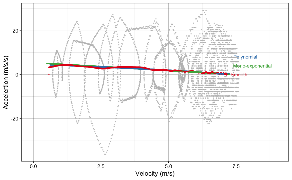
(a) Estimated AVP using raw velocity and raw acceleration

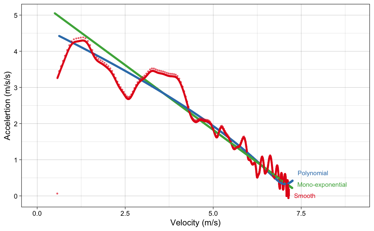
(b) Estimated AVP using model predicted velocity and acceleration

Figure 5: Acceleration-Velocity Profile (AVP)

Please note that there is no “profile” when using raw velocity and acceleration estimated from raw velocity (grey dots in Figure 5 (a)). The key thing to notice from Figure 5 (b), is that AVP for the mono-exponential model is linear. This is indeed interesting characteristic of this model, since with only two parameters (i.e., MSS and MAC or TAU) we can explain the whole profile. It is indeed mathematically elegant model.

Kinetics and Force-Velocity Profile

To create Force-Velocity Profile (FVP), we simply need to estimate the total step average force being generated horizontally by the athlete. Since we know the instant acceleration and athlete body mass, we can calculate the net force, by simply multiplying the weight with acceleration. But athlete also needs to overcome one more force (i.e., one more force according to this simple model; there are multiple other forces and work that needs to be done to move the limbs, as alluded previously): air resistance force. Air resistance force (measured in Newtons, N) depends on the velocity, body mass (kg), body height (m), barometric pressure (Torr), air temperature ($ C^\circ $), and wind velocity ($ ms^-1 $) (please refer to Arsac and Locatelli (2002), P. Samozino et al. (2016), and Ingen Schenau, Jacobs, and Koning (1991) for more information).

We can simply estimate total horizontal force by using $ F_{total} = a \times m + F_{air} $ by assuming athlete weights 85kg and is tall 1.8m (see the code for Figure 6).

# Add air resistance
laser_models_df <- laser_models_df %>%
  mutate(
    f_air = get_air_resistance(velocity = velocity, bodymass = 85,  bodyheight = 1.8),
    f_total = 85 * acceleration + f_air,
    f_total_relative = f_total / 85,
    power = f_total * velocity,
    relative_power = power / 85
    )

ggplot(
  laser_models_df %>% 
    filter(model != "Raw-Velocity"),
  aes(x = velocity, y = f_total, color = model)) +
  theme_linedraw(8) +
  geom_point(
    data = laser_models_df %>% 
    filter(model == "Raw-Velocity"), 
    aes(x = velocity, y = f_total),
    color = "grey",
    size = 0.05,
    alpha = 0.8
  ) +
  geom_point(alpha = 0.5, size = 0.25) +
  scale_color_brewer(palette = "Set1") +
  xlab("Velocity (m/s)") +
  ylab("Horizontal Force (N)") +
  theme(legend.position = "none") +
  geom_dl(
    aes(label = paste("  ", model)),
    method = list("last.bumpup", cex = 0.5)
  ) +
  xlim(0, 9)

ggplot(
  laser_models_df %>% 
    filter(model != "Raw-Velocity"),
  aes(x = velocity, y = f_total, color = model)) +
  theme_linedraw(8) +
  geom_point(alpha = 0.5, size = 0.25) +
  scale_color_brewer(palette = "Set1") +
  xlab("Velocity (m/s)") +
  ylab("Horizontal Force (N)") +
  theme(legend.position = "none") +
  geom_dl(
    aes(label = paste("  ", model)),
    method = list("last.bumpup", cex = 0.5)
  ) +
  xlim(0, 9)

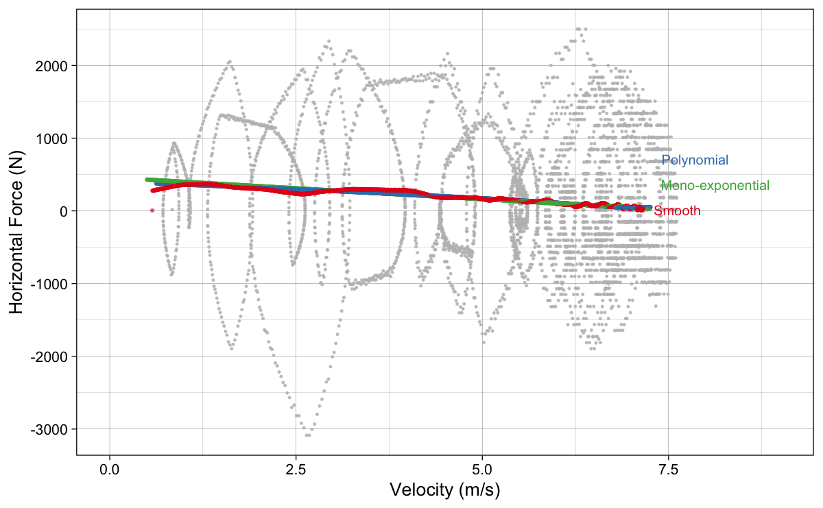
(a) Estimated FVP using raw velocity, raw acceleration, and air resistance

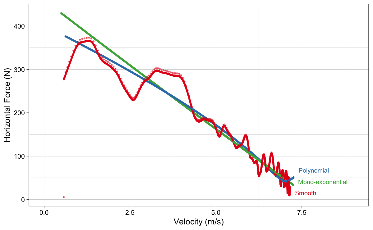
(b) Estimated FVP using model predicted velocity, acceleration, and air resistance

Figure 6: Force-Velocity Profile (FVP)

As can be seen, the shape of Figure 6 (b) is very similar to Figure 5. One thing to notice, although a bit harder, is that FVP for the mono-exponential model is not a straight line anymore, but very, very close to being straight. We can thus act-as-if it is straight line. But this will introduce some error, as I will explore in the next installment.

Now when we have total horizontal force, we can also calculate total power (Figure 7). This is power used to gain horizontal momentum and to overcome air resistance, but not exactly the total power needed to move the limbs, overcome vertical up and down movements and so forth.

# Plot net relative power
ggplot(
  laser_models_df %>% 
    filter(model != "Raw-Velocity"),
  aes(x = Time, y = power, color = model)) +
  theme_linedraw(8) +
  geom_line(
    data = laser_models_df %>% 
    filter(model == "Raw-Velocity"), 
    aes(x = Time, y = power),
    color = "grey",
    alpha = 0.8
  ) +
  geom_line(alpha = 0.8) +
  scale_color_brewer(palette = "Set1") +
  xlab("Time (sec)") +
  ylab("Power (W)") +
  theme(legend.position = "none") +
  geom_dl(
    aes(label = paste("  ", model)),
    method = list("last.bumpup", cex = 0.5)
  ) +
  xlim(0, 5.5)

ggplot(
  laser_models_df %>% 
    filter(model != "Raw-Velocity"),
  aes(x = Time, y = power, color = model)) +
  theme_linedraw(8) +
  geom_line(alpha = 0.8) +
  scale_color_brewer(palette = "Set1") +
  xlab("Time (sec)") +
  ylab("Power (W)") +
  theme(legend.position = "none") +
  geom_dl(
    aes(label = paste("  ", model)),
    method = list("last.bumpup", cex = 0.5)
  ) +
  xlim(0, 5.5)

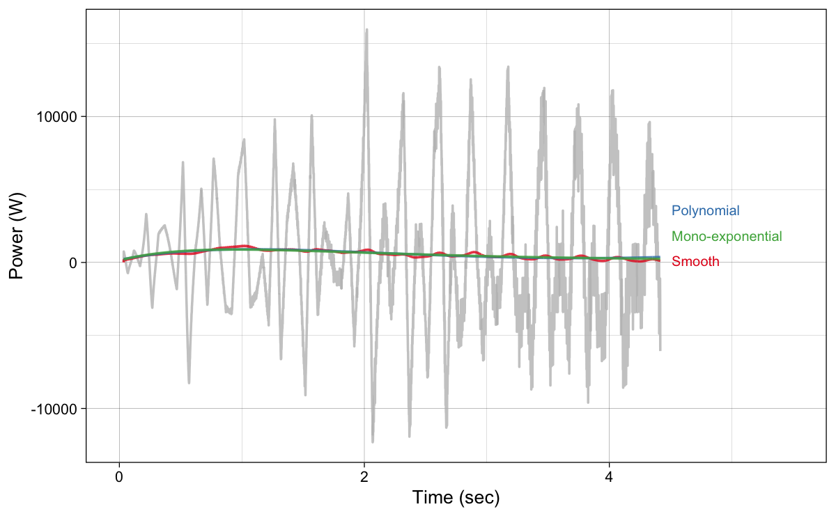
(a) Estimated FVP using raw velocity, raw acceleration, and air resistance

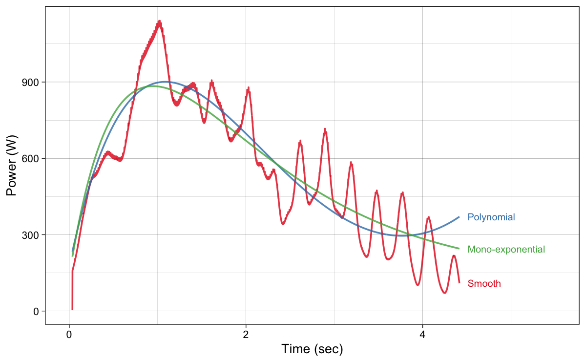
(a) Estimated FVP using raw velocity, raw acceleration, and air resistance

Figure 7: Estimated total power using horizontal force x velocity

Key takeways

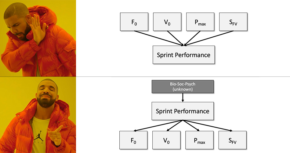
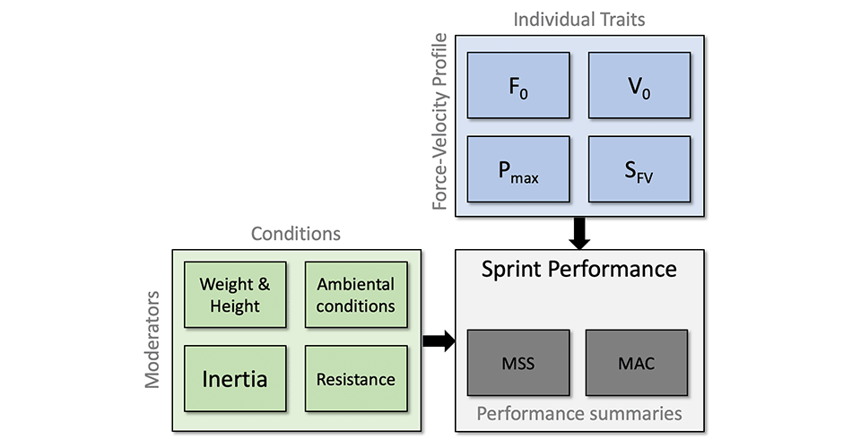
In my opinion, the models introduced here serve to simplify or summarize the observed sprint performance, rather than to uncover some hidden causal qualities (i.e., traits). There are a lot of assumptions and probably a lot of useful information being disregarded (e.g., total power generated, within step acceleration and deceleration fluctuations) to create simplistic summaries these models provide. But they can be useful for that purpose, as long as we do not give them more (causal) power and interpretation. I will expand on these topics thorough this article series.

As seen in this first installment, mono-exponential model seems like a more favorable model to describe short sprints: it is more theoretical aligned with out expectations, it is mathematically more elegant, and it also provides parameters (i.e., MSS, TAU, MAC) that are more interpretable and more related to the real traits/qualities, or at least to the phenomena we observe (e.g., someone being better accelerator will have higher MAC parameter values).

In the next installment I will continue with exploring the characteristics of the mono-exponential model. Although velocity trace acquired from the radar/laser gun can be more telling, we often do not have access to those, and must use timing gates. But we can still use variant of the mono-exponential model to estimate MSS and TAU parameters, and using those to create AVP and FVP, as well as play with model optimization.

In the next installment I will explore the assumptions and behavior of the mono-exponential model itself, which is needed to understand the concept of optimal FVP for sprinting. It is important to keep in mind that these are characteristics of the “Small World” model, rather than characteristics of the “Large World” - please do not confuse model for the reality. Map is not the territory.

References

1. Arsac, Laurent M., and Elio Locatelli. 2002. “Modeling the Energetics of 100-m Running by Using Speed Curves of World Champions.” Journal of Applied Physiology 92 (5): 1781–88. https://doi.org/10.1152/japplphysiol.00754.2001.
2. Binmore, Ken. 2011. Rational Decisions. Fourth Impression edition. Princeton, NJ: Princeton University Press.
3. Gigerenzer, Gerd, Ralph Hertwig, and Thorsten Pachur. 2015. Heuristics: The Foundations of Adaptive Behavior. Reprint edition. Oxford University Press.
4. Ingen Schenau, Gerrit Jan van, Ron Jacobs, and Jos J. de Koning. 1991. “Can Cycle Power Predict Sprint Running Performance?” European Journal of Applied Physiology and Occupational Physiology 63 (3-4): 255–60. https://doi.org/10.1007/BF00233857.
5. Jovanović, Mladen. 2020. Strength Training Manual: The Agile Periodization Approach. Independently published.
6. ———. 2022. Shorts: Short Sprints. https://cran.r-project.org/package=shorts.
7. Jovanović, Mladen, and Jason Vescovi. 2022. “Shorts: An r Package for Modeling Short Sprints.” International Journal of Strength and Conditioning 2 (1). https://doi.org/10.47206/ijsc.v2i1.74.
8. McElreath, Richard. 2020. Statistical Rethinking: A Bayesian Course with Examples in r and Stan. 2nd ed. CRC Texts in Statistical Science. Boca Raton: Taylor; Francis, CRC Press.
9. R Core Team. 2022. R: A Language and Environment for Statistical Computing. Vienna, Austria: R Foundation for Statistical Computing. https://www.R-project.org/.
10. Samozino, P., P. Edouard, S. Sangnier, M. Brughelli, P. Gimenez, and J.-B. Morin. 2013. “Force-Velocity Profile: Imbalance Determination and Effect on Lower Limb Ballistic Performance.” International Journal of Sports Medicine 35 (06): 505–10. https://doi.org/10.1055/s-0033-1354382.
11. Samozino, Pierre. 2018. “Optimal Force-Velocity Profile in Ballistic Push-Off: Measurement and Relationship with Performance.” In, edited by Jean-Benoit Morin and Pierre Samozino, 97–119. Cham: Springer International Publishing. https://doi.org/10.1007/978-3-319-05633-3_5.
12. Samozino, Pierre, Jean-Benoît Morin, Frédérique Hintzy, and Alain Belli. 2008. “A Simple Method for Measuring Force, Velocity and Power Output During Squat Jump.” Journal of Biomechanics 41 (14): 2940–45. https://doi.org/10.1016/j.jbiomech.2008.07.028.
13. Samozino, Pierre, Nicolas Peyrot, Pascal Edouard, Ryu Nagahara, Pedro Jimenez-Reyes, Benedicte Vanwanseele, and Jean-Benoit Morin. 2022. “Optimal Mechanical Force-Velocity Profile for Sprint Acceleration Performance.” Scandinavian Journal of Medicine & Science in Sports 32 (3): 559–75. https://doi.org/10.1111/sms.14097.
14. Samozino, Pierre, Enrico Rejc, Pietro Enrico Di Prampero, Alain Belli, and Jean-Benoît Morin. 2012. “Optimal ForceVelocity Profile in Ballistic MovementsAltius:” Medicine & Science in Sports & Exercise 44 (2): 313–22. https://doi.org/10.1249/MSS.0b013e31822d757a.
15. Samozino, P., G. Rabita, S. Dorel, J. Slawinski, N. Peyrot, E. Saez de Villarreal, and J.-B. Morin. 2016. “A Simple Method for Measuring Power, Force, Velocity Properties, and Mechanical Effectiveness in Sprint Running: Simple Method to Compute Sprint Mechanics.” Scandinavian Journal of Medicine & Science in Sports 26 (6): 648–58. https://doi.org/10.1111/sms.12490.
16. Savage, Leonard J. 1972. The Foundations of Statistics. 2nd Revised ed. edition. New York: Dover Publications.
17. Volz, Kirsten G, and Gerd Gigerenzer. 2012. “Cognitive Processes in Decisions Under Risk Are Not the Same as in Decisions Under Uncertainty.” Frontiers in Neuroscience 6 (105). https://doi.org/10.3389/fnins.2012.00105.

Footnotes

1. You can find more about this model and my beef with it in the Force-Velocity Profiling and Training Optimization Course ↩︎