What Is Propensity Matching and How Can We Improve Validity of Causality Claims?
Introduction
It is generaly hard to do randomized trial in performance environment, especially with higher-level athletes. It is a gold standard method that tries to minimize confounders (although they do happen as I will demonstrate) between control and treatment groups, so the effects could be assigned to the treatment and not something else (confounders). This allows for certainty in making causal claims (Treatment A cause effects B).
But can we do same with observational studies and data? Less likely, since we are not controlling (by the design) all the potential confounders that might influence the effects and hence reduce the confidence in causal claims. They are easier to do though. Much easier. But can we do something about it? Reading Data Analysis Using Regression and Multilevel/Hierarchical Models, which is must have book btw, gave me couple of ideas/solutions that I want to explore in this post. So, yes this is a playbook, and I am hoping it will give you some food for thought and practical tools for data analysis.
Data set
For the purpose of this playbook, I created data set that represents hypothetical randomized trial of novel periodization method. We are interested in the effects of new periodization method to the increase in back squat 1RM.
We have 100 subjects, evenly split into control and treatment group, whose 1RM back squat is measured before and after treatment. Subject characteristics include training age, body weight and pre-test 1RM. By randomizing we want to make sure that the control and treatment groups are not-significantly different in those characteristic.
Here is the data generation script:
# Set random number generator seed so you can reproduce the scores
set.seed(1982)

athletesNumber = 100

# Generate group (Control/Treatment)
group <- gl(n = 2, length = athletesNumber,
          k = 1, labels = c("Control", "Treatment"))

# Generate Age
ageTraining <- round(rnorm(n = athletesNumber, mean= 10, sd = 2), 0)

# Generate BW
bodyWeight <- round(rnorm(n = athletesNumber, mean= 80, sd = 10), 0)

# Pretest squat 1RM
preTestSquat1RM <- round(1.5 * ageTraining + 1.5 * bodyWeight +
                        rnorm(n = athletesNumber, mean= 0, sd = 10), 0)

# Intervention training volume (Arbitrary number)
trainingVolume <- round(100 + ifelse(group == "Treatment",
                                     15 + rnorm(n = athletesNumber, mean= 0, sd = 15),
                                     0 +  rnorm(n = athletesNumber, mean= 0, sd = 8)), 0)

# Posttest squat 1RM
postTestSquat1RM <- round(1.1 * preTestSquat1RM +
                          0.15 * trainingVolume +
                          ifelse(group == "Treatment", 4, 0) +
                          rnorm(n = athletesNumber, mean= 0, sd = 8), 0)

# Difference
difference <- postTestSquat1RM - preTestSquat1RM

# Percent change
change <- round(difference / preTestSquat1RM, 2)

# Save the data in data frame
studyData <- data.frame(ageTraining,
                        bodyWeight,
                        preTestSquat1RM,
                        group,
                        trainingVolume,
                        postTestSquat1RM,
                        difference,
                        change)
Let’s plot the data. Each dot represent a subject (they are “jittered” for easier viewing). The vertical line and a dot represent mean and 1 SD.
suppressPackageStartupMessages(library(ggplot2))
suppressPackageStartupMessages(library(reshape2))

# Convert to long format for plotting
studyDataLong <- melt(studyData, id.vars = "group")

gg <- ggplot(studyDataLong, aes(x = group, y = value, color = group)) +
      geom_jitter(alpha = 0.3, width = 0.4) +
      stat_summary(geom = "pointrange", fun.data = "mean_sdl",
                   size = 0.4, color = "black") +
      facet_wrap(~variable, scales = "free") +
      theme_bw() +
      theme(legend.position="none")
print(gg)
As can be seen from the graph there is not much difference between Control and Treatment group in trainign age, body weight and pre test 1RM. So far so good. There is some difference between training volume (arbitary number) and of course between training effects: post test 1RM, difference and change.
Let’s perform t-test on each parameter to check if the differences between control and treatment groups are statistically significant:
lapply(studyData[-4], function(x) t.test(x ~ studyData$group))## $ageTraining
##
## Welch Two Sample t-test
##
## data: x by studyData$group
## t = -0.049943, df = 97.924, p-value = 0.9603
## alternative hypothesis: true difference in means is not equal to 0
## 95 percent confidence interval:
## -0.8147054 0.7747054
## sample estimates:
## mean in group Control mean in group Treatment
## 10.02 10.04
##
##
## $bodyWeight
##
## Welch Two Sample t-test
##
## data: x by studyData$group
## t = -1.4167, df = 96.951, p-value = 0.1598
## alternative hypothesis: true difference in means is not equal to 0
## 95 percent confidence interval:
## -6.146431 1.026431
## sample estimates:
## mean in group Control mean in group Treatment
## 80.04 82.60
##
##
## $preTestSquat1RM
##
## Welch Two Sample t-test
##
## data: x by studyData$group
## t = -1.4886, df = 97.773, p-value = 0.1398
## alternative hypothesis: true difference in means is not equal to 0
## 95 percent confidence interval:
## -10.685656 1.525656
## sample estimates:
## mean in group Control mean in group Treatment
## 134.84 139.42
##
##
## $trainingVolume
##
## Welch Two Sample t-test
##
## data: x by studyData$group
## t = -5.3087, df = 75.164, p-value = 1.081e-06
## alternative hypothesis: true difference in means is not equal to 0
## 95 percent confidence interval:
## -18.483205 -8.396795
## sample estimates:
## mean in group Control mean in group Treatment
## 100.38 113.82
##
##
## $postTestSquat1RM
##
## Welch Two Sample t-test
##
## data: x by studyData$group
## t = -2.6192, df = 97.628, p-value = 0.01022
## alternative hypothesis: true difference in means is not equal to 0
## 95 percent confidence interval:
## -17.577058 -2.422942
## sample estimates:
## mean in group Control mean in group Treatment
## 165.02 175.02
##
##
## $difference
##
## Welch Two Sample t-test
##
## data: x by studyData$group
## t = -3.4723, df = 91.573, p-value = 0.0007896
## alternative hypothesis: true difference in means is not equal to 0
## 95 percent confidence interval:
## -8.520321 -2.319679
## sample estimates:
## mean in group Control mean in group Treatment
## 30.18 35.60
##
##
## $change
##
## Welch Two Sample t-test
##
## data: x by studyData$group
## t = -2.6219, df = 82.393, p-value = 0.01041
## alternative hypothesis: true difference in means is not equal to 0
## 95 percent confidence interval:
## -0.052760283 -0.007239717
## sample estimates:
## mean in group Control mean in group Treatment
## 0.2262 0.2562We can also perform bootstraped Effect Size (ES; Cohen’s D) calculation:
suppressPackageStartupMessages(library(bootES))

lapply(studyData[-4], function(x) {bootES(data.frame(param = x, group = studyData$group),
                                      data.col = "param",
                                      group.col = "group",
                                      contrast = c("Control", "Treatment"),
                                      effect.type = "cohens.d")})
## $ageTraining
##
## User-specified lambdas: (Control, Treatment)
## Scaled lambdas: (-1, 1)
## 95.00% bca Confidence Interval, 2000 replicates
## Stat CI (Low) CI (High) bias SE
## 0.010 -0.400 0.416 -0.007 0.204
##
##
## $bodyWeight
##
## User-specified lambdas: (Control, Treatment)
## Scaled lambdas: (-1, 1)
## 95.00% bca Confidence Interval, 2000 replicates
## Stat CI (Low) CI (High) bias SE
## 0.283 -0.128 0.691 0.004 0.210
##
##
## $preTestSquat1RM
##
## User-specified lambdas: (Control, Treatment)
## Scaled lambdas: (-1, 1)
## 95.00% bca Confidence Interval, 2000 replicates
## Stat CI (Low) CI (High) bias SE
## 0.298 -0.122 0.681 0.011 0.206
##
##
## $trainingVolume
##
## User-specified lambdas: (Control, Treatment)
## Scaled lambdas: (-1, 1)
## 95.00% bca Confidence Interval, 2000 replicates
## Stat CI (Low) CI (High) bias SE
## 1.062 0.627 1.455 0.020 0.207
##
##
## $postTestSquat1RM
##
## User-specified lambdas: (Control, Treatment)
## Scaled lambdas: (-1, 1)
## 95.00% bca Confidence Interval, 2000 replicates
## Stat CI (Low) CI (High) bias SE
## 0.524 0.110 0.948 0.013 0.212
##
##
## $difference
##
## User-specified lambdas: (Control, Treatment)
## Scaled lambdas: (-1, 1)
## 95.00% bca Confidence Interval, 2000 replicates
## Stat CI (Low) CI (High) bias SE
## 0.694 0.286 1.117 0.011 0.208
##
##
## $change
##
## User-specified lambdas: (Control, Treatment)
## Scaled lambdas: (-1, 1)
## 95.00% bca Confidence Interval, 2000 replicates
## Stat CI (Low) CI (High) bias SE
## 0.524 0.089 0.950 0.016 0.215As can be seen from the ES, the differences between control and treatment in training age, body weight and pre-test squat 1RM are very small and their CIs include zero (hence they are non-significant). That is not the case with training volume, post-test 1RM, difference and percent change.
Analysis
As a researchers and coaches we might be interested in the effects of this novel periodization on the changes in back squat 1RMs (in the population; inference or generalization). To do this we can perform ANOVA or linear regression. I preffer linear regression approach (the results are the same):
model1 <- lm(difference ~ group, studyData)
summary(model1)
##
## Call:
## lm(formula = difference ~ group, data = studyData)
##
## Residuals:
## Min 1Q Median 3Q Max
## -15.18 -6.60 -0.60 5.82 16.40
##
## Coefficients:
## Estimate Std. Error t value Pr(>|t|)
## (Intercept) 30.180 1.104 27.343 < 2e-16 ***
## groupTreatment 5.420 1.561 3.472 0.000769 ***
## ---
## Signif. codes: 0 '***' 0.001 '**' 0.01 '*' 0.05 '.' 0.1 ' ' 1
##
## Residual standard error: 7.805 on 98 degrees of freedom
## Multiple R-squared: 0.1096, Adjusted R-squared: 0.1005
## F-statistic: 12.06 on 1 and 98 DF, p-value: 0.0007694confint(model1)## 2.5 % 97.5 %
## (Intercept) 27.989665 32.370335
## groupTreatment 2.322398 8.517602And we can conclude that effect of this novel periodization method is statistically significant.
But what we didn’t take into account is the training volume. We can plug training volume into the regression formula as interaction, but before that let’s plot scatterplot of training volume and difference change in 1RM:
gg <- ggplot(studyData, aes(x = trainingVolume,
                            y = difference,
                            color = group,
                            fill = group)) +
      geom_smooth(alpha = 0.1, method = "lm") +
      geom_point(alpha = 0.6) +
      theme_bw() +
      theme(legend.position="top")
print(gg)
They do seem to overlap, where the threatment group have much bigger spread and higher mean. The do seem to have slope (effect) of same size, which can be that the treatment is NOT what is affecting the changes in 1RM.
Let’s do regression analysis and see if the effects of training volume are significant. First we are going to perform linear regression regardless of the group (i.e. pooled):
model2 <- lm(difference ~ trainingVolume, studyData)
summary(model2)
##
## Call:
## lm(formula = difference ~ trainingVolume, data = studyData)
##
## Residuals:
## Min 1Q Median 3Q Max
## -16.3498 -5.6979 0.2872 5.3213 13.8602
##
## Coefficients:
## Estimate Std. Error t value Pr(>|t|)
## (Intercept) 6.97126 5.70225 1.223 0.224
## trainingVolume 0.24201 0.05278 4.585 1.34e-05 ***
## ---
## Signif. codes: 0 '***' 0.001 '**' 0.01 '*' 0.05 '.' 0.1 ' ' 1
##
## Residual standard error: 7.505 on 98 degrees of freedom
## Multiple R-squared: 0.1766, Adjusted R-squared: 0.1682
## F-statistic: 21.02 on 1 and 98 DF, p-value: 1.34e-05confint(model2)## 2.5 % 97.5 %
## (Intercept) -4.3446661 18.2871856
## trainingVolume 0.1372666 0.3467435This is the control group:
model3 <- lm(difference ~ trainingVolume, subset(studyData, group == "Control"))
summary(model3)
##
## Call:
## lm(formula = difference ~ trainingVolume, data = subset(studyData,
## group == "Control"))
##
## Residuals:
## Min 1Q Median 3Q Max
## -15.1996 -7.4195 0.3462 5.6633 14.0805
##
## Coefficients:
## Estimate Std. Error t value Pr(>|t|)
## (Intercept) 6.6622 14.6587 0.454 0.652
## trainingVolume 0.2343 0.1455 1.610 0.114
##
## Residual standard error: 8.639 on 48 degrees of freedom
## Multiple R-squared: 0.05123, Adjusted R-squared: 0.03147
## F-statistic: 2.592 on 1 and 48 DF, p-value: 0.114confint(model3)## 2.5 % 97.5 %
## (Intercept) -22.81116459 36.1354697
## trainingVolume -0.05830778 0.5268841And for the treatment group:
model4 <- lm(difference ~ trainingVolume, subset(studyData, group == "Treatment"))
summary(model4)
##
## Call:
## lm(formula = difference ~ trainingVolume, data = subset(studyData,
## group == "Treatment"))
##
## Residuals:
## Min 1Q Median 3Q Max
## -12.2643 -4.7499 -0.0554 3.8668 12.8624
##
## Coefficients:
## Estimate Std. Error t value Pr(>|t|)
## (Intercept) 14.60671 6.33869 2.304 0.02557 *
## trainingVolume 0.18444 0.05517 3.343 0.00161 **
## ---
## Signif. codes: 0 '***' 0.001 '**' 0.01 '*' 0.05 '.' 0.1 ' ' 1
##
## Residual standard error: 6.089 on 48 degrees of freedom
## Multiple R-squared: 0.1888, Adjusted R-squared: 0.1719
## F-statistic: 11.18 on 1 and 48 DF, p-value: 0.001614confint(model4)## 2.5 % 97.5 %
## (Intercept) 1.86191093 27.3515104
## trainingVolume 0.07350768 0.2953781What if we plug in the training volume as interaction (pretty much ANCOVA) with group? Will it decrease the effects of the treatment?
model5 <- lm(difference ~ trainingVolume*group, studyData)
summary(model5)
##
## Call:
## lm(formula = difference ~ trainingVolume * group, data = studyData)
##
## Residuals:
## Min 1Q Median 3Q Max
## -15.1996 -5.5512 0.1535 5.5368 14.0805
##
## Coefficients:
## Estimate Std. Error t value Pr(>|t|)
## (Intercept) 6.66215 12.68145 0.525 0.6006
## trainingVolume 0.23429 0.12589 1.861 0.0658 .
## groupTreatment 7.94456 14.87760 0.534 0.5946
## trainingVolume:groupTreatment -0.04985 0.14295 -0.349 0.7281
## ---
## Signif. codes: 0 '***' 0.001 '**' 0.01 '*' 0.05 '.' 0.1 ' ' 1
##
## Residual standard error: 7.473 on 96 degrees of freedom
## Multiple R-squared: 0.2002, Adjusted R-squared: 0.1752
## F-statistic: 8.011 on 3 and 96 DF, p-value: 8.068e-05confint(model5)## 2.5 % 97.5 %
## (Intercept) -18.51032362 31.8346288
## trainingVolume -0.01561124 0.4841876
## groupTreatment -21.58725017 37.4763664
## trainingVolume:groupTreatment -0.33360203 0.2339114As can be seen the model perform better (lower residual standar error), but now the effect of treatment is not statistically significant.
Propensity Score matching
Another approach, besides plugging covariates into the regression together with the group variable, is matching.
Sometimes the randomized assignment to groups doesn’t result in equal groups. This is more common in observational studies. What we are looking to do is to “match” the individuals, or in other words find the pairs of individuals (or observations) in each group (control and treatment) that have similar characteristics (covariates). Usually, covariates are “pre intervention” variables, but as seen above I’ve used training volume as covariate as well.
How to do this? One method is to use “propensity scores”. Propensity score in nothing more than probability of being in treatment group. This is usually done with logistic regression, where we want to predict the group of the individual based on his covariates.
Let’s do it with out data, utilizing training age, body weight and pre test 1RM in this case:
propensityModel1 <- glm(group ~ ageTraining + bodyWeight + preTestSquat1RM,
                       studyData,
                       family = "binomial")

studyData$propensityScore1 <- predict(propensityModel1, type = "response")
If we plot the distribution of propensity scores across group we want to see overlap. Overlap means that individuals have same/similar probability being in either group based on the covariates. That is exactly what we want with randomized trial.
gg <- ggplot(studyData, aes(x = propensityScore1, fill = group)) +
      geom_density(alpha = 0.5) +
      theme_bw()

print(gg)
As can be seen there is an overlap. We can perform t-test on propensity score to check if the groups differ
t.test(propensityScore1 ~ group, studyData)##
## Welch Two Sample t-test
##
## data: propensityScore1 by group
## t = -1.6148, df = 96.045, p-value = 0.1096
## alternative hypothesis: true difference in means is not equal to 0
## 95 percent confidence interval:
## -0.057181903 0.005879697
## sample estimates:
## mean in group Control mean in group Treatment
## 0.4871744 0.5128256As can be seen the difference is not statistically significant. This mean that we performed randomization correctly.
But what if we enter training volume into the equation?
propensityModel2 <- glm(group ~ ageTraining + bodyWeight +
                                preTestSquat1RM + trainingVolume,
                       studyData,
                       family = "binomial")

studyData$propensityScore2 <- predict(propensityModel2, type = "response")

gg <- ggplot(studyData, aes(x = propensityScore2, fill = group)) +
      geom_density(alpha = 0.5) +
      theme_bw()

print(gg)
There is less overlap. This is troublesome because this means that our groups are not randomized correctly. Let’s perform t-test
t.test(propensityScore2 ~ group, studyData)##
## Welch Two Sample t-test
##
## data: propensityScore2 by group
## t = -5.4355, df = 84.328, p-value = 5.214e-07
## alternative hypothesis: true difference in means is not equal to 0
## 95 percent confidence interval:
## -0.3174002 -0.1473701
## sample estimates:
## mean in group Control mean in group Treatment
## 0.3838074 0.6161926And as can be expected, the propensity score between groups significantly differs.
What can we do? Well, we can perform matching. Matching is trying to find pairs of subjects (from each group) that are most similar in propensity score. There are multiple algorythms to do this and I with use MatchIt.
suppressPackageStartupMessages(library(MatchIt))

# Convert group to 0 = Control, 1 = Treatment as needed by matchit function
studyData$treatment = ifelse(studyData$group == "Treatment", 1, 0)

m <- matchit(treatment ~ ageTraining + bodyWeight +
                         preTestSquat1RM + trainingVolume,
             data = studyData,
             method = "nearest",
             discard = "both")
print(m)
##
## Call:
## matchit(formula = treatment ~ ageTraining + bodyWeight + preTestSquat1RM +
## trainingVolume, data = studyData, method = "nearest", discard = "both")
##
## Sample sizes:
## Control Treated
## All 50 50
## Matched 31 31
## Unmatched 18 0
## Discarded 1 19Let’s calculate our propensity scores again after matching and plot it:
matched <- match.data(m)

propensityModel3 <- glm(group ~ ageTraining + bodyWeight +
                                preTestSquat1RM + trainingVolume,
                       matched,
                       family = "binomial")

matched$propensityScore <- predict(propensityModel3, type = "response")

gg <- ggplot(matched, aes(x = propensityScore, fill = group)) +
      geom_density(alpha = 0.5) +
      theme_bw()

print(gg)
As can be seen there is an overlap now. Let’s plot the distributions as we did at the beginning, but now using matched subjects:
# Convert to long format for plotting
macthedLong <- melt(matched[1:8], id.vars = "group")

gg <- ggplot(macthedLong, aes(x = group, y = value, color = group)) +
      geom_jitter(alpha = 0.3, width = 0.4) +
      stat_summary(geom = "pointrange", fun.data = "mean_sdl",
                   size = 0.4, color = "black") +
      facet_wrap(~variable, scales = "free") +
      theme_bw() +
      theme(legend.position="none")
print(gg)
As it seems now, the training volume is much more similar between groups than before matching.
We can plot the relationship of training volume to change scores as we did before:
gg <- ggplot(matched, aes(x = trainingVolume,
                            y = difference,
                            color = group,
                            fill = group)) +
      geom_smooth(alpha = 0.1, method = "lm") +
      geom_point(alpha = 0.6) +
      theme_bw() +
      theme(legend.position="top")
print(gg)
As can be seen they pretty much overlap, which is the goal of matching.
Let’s do linear regression to judge the effects:
matchedModel1 <- lm(difference ~ group, matched)
summary(matchedModel1)
##
## Call:
## lm(formula = difference ~ group, data = matched)
##
## Residuals:
## Min 1Q Median 3Q Max
## -15.9677 -4.7742 -0.6935 5.0323 14.0323
##
## Coefficients:
## Estimate Std. Error t value Pr(>|t|)
## (Intercept) 30.968 1.398 22.156 <2e-16 ***
## groupTreatment 2.226 1.977 1.126 0.265
## ---
## Signif. codes: 0 '***' 0.001 '**' 0.01 '*' 0.05 '.' 0.1 ' ' 1
##
## Residual standard error: 7.782 on 60 degrees of freedom
## Multiple R-squared: 0.02069, Adjusted R-squared: 0.004373
## F-statistic: 1.268 on 1 and 60 DF, p-value: 0.2646confint(matchedModel1)## 2.5 % 97.5 %
## (Intercept) 28.17186 33.763626
## groupTreatment -1.72817 6.179783If we compare it the un-matched data:
model1 <- lm(difference ~ group, studyData)
summary(model1)
##
## Call:
## lm(formula = difference ~ group, data = studyData)
##
## Residuals:
## Min 1Q Median 3Q Max
## -15.18 -6.60 -0.60 5.82 16.40
##
## Coefficients:
## Estimate Std. Error t value Pr(>|t|)
## (Intercept) 30.180 1.104 27.343 < 2e-16 ***
## groupTreatment 5.420 1.561 3.472 0.000769 ***
## ---
## Signif. codes: 0 '***' 0.001 '**' 0.01 '*' 0.05 '.' 0.1 ' ' 1
##
## Residual standard error: 7.805 on 98 degrees of freedom
## Multiple R-squared: 0.1096, Adjusted R-squared: 0.1005
## F-statistic: 12.06 on 1 and 98 DF, p-value: 0.0007694confint(model1)## 2.5 % 97.5 %
## (Intercept) 27.989665 32.370335
## groupTreatment 2.322398 8.517602We can see that there is a huge difference, and that matching subjects yielded much smaller effect of the treatment. Pretty much the cause is different training volume and not the intervention.
Let’s compare models with interaction. Here is matched:
matchedModel2 <- lm(difference ~ group*trainingVolume, matched)
summary(matchedModel2)
##
## Call:
## lm(formula = difference ~ group * trainingVolume, data = matched)
##
## Residuals:
## Min 1Q Median 3Q Max
## -16.0647 -4.7075 -0.0358 4.7694 12.9007
##
## Coefficients:
## Estimate Std. Error t value Pr(>|t|)
## (Intercept) -2.0131 16.4268 -0.123 0.9029
## groupTreatment 12.7240 21.8811 0.582 0.5632
## trainingVolume 0.3218 0.1597 2.015 0.0486 *
## groupTreatment:trainingVolume -0.1056 0.2114 -0.500 0.6191
## ---
## Signif. codes: 0 '***' 0.001 '**' 0.01 '*' 0.05 '.' 0.1 ' ' 1
##
## Residual standard error: 7.506 on 58 degrees of freedom
## Multiple R-squared: 0.1194, Adjusted R-squared: 0.07382
## F-statistic: 2.621 on 3 and 58 DF, p-value: 0.05925confint(matchedModel2)## 2.5 % 97.5 %
## (Intercept) -34.894971896 30.8688176
## groupTreatment -31.075906613 56.5238280
## trainingVolume 0.002047561 0.6415819
## groupTreatment:trainingVolume -0.528698476 0.3174280And here is our original un-matched data set:
model5 <- lm(difference ~ trainingVolume*group, studyData)
summary(model5)
##
## Call:
## lm(formula = difference ~ trainingVolume * group, data = studyData)
##
## Residuals:
## Min 1Q Median 3Q Max
## -15.1996 -5.5512 0.1535 5.5368 14.0805
##
## Coefficients:
## Estimate Std. Error t value Pr(>|t|)
## (Intercept) 6.66215 12.68145 0.525 0.6006
## trainingVolume 0.23429 0.12589 1.861 0.0658 .
## groupTreatment 7.94456 14.87760 0.534 0.5946
## trainingVolume:groupTreatment -0.04985 0.14295 -0.349 0.7281
## ---
## Signif. codes: 0 '***' 0.001 '**' 0.01 '*' 0.05 '.' 0.1 ' ' 1
##
## Residual standard error: 7.473 on 96 degrees of freedom
## Multiple R-squared: 0.2002, Adjusted R-squared: 0.1752
## F-statistic: 8.011 on 3 and 96 DF, p-value: 8.068e-05confint(model5)## 2.5 % 97.5 %
## (Intercept) -18.51032362 31.8346288
## trainingVolume -0.01561124 0.4841876
## groupTreatment -21.58725017 37.4763664
## trainingVolume:groupTreatment -0.33360203 0.2339114The coefficients are pretty similar, but the effect of training volume is even higher in matched group
Conclusion
Researchers usually try to randomize correctly, but sometimes the effect is not in the treatment, but maybe in the differnce between group (pre-treatment) or during the treatment (for example volume of training) which should be similar/same so we can judge the effects of something else of interest (for example novel periodization). The solutions are to involve covariates in the model and/or do the matching. Sometimes the number of subject is so small, so the matching is out of question (but it is really interesting tool with observational data where we might have much more subjects/observatoins).
Hence next time when you read that the new periodization or any other treatment is statistically significant, make sure to read the methods and statistical analysis as well.
Hope this example gave you some ideas and practical tools you can use.


Responses