Velocity-Based Training: Signal vs. Noise
This is a R workbook using my older bench press data, in which I want to discuss Signal vs. Noise of Velocity-Based Training (VBT) measurements. This could be used for future reliability studies. The goal is to compare within-individual variations of velocity over load-velocity relationship (noise) with smallest practical velocity difference (in my opinion difference in velocities across nRM, e.g. 4RM – 5RM) which could be called signal
Data
I have saved some of my old data in .CSV file (originaly published at GymAware website). The data represents mean velocity (MV) of bench press (sets of 1 rep) at 4 intensity levels (40, 60, 80 and 100kg), performed for three sets each (with 3sec pause on the chest). N = 1 (the author)
# Load data
VBT.1RM.data <- read.csv("1RM test velocity.csv", header = TRUE)| Exercise | Load | Set | Velocity | |
|---|---|---|---|---|
| 1 | Bench | 40 | 1 | 1.00 |
| 2 | Bench | 40 | 2 | 1.01 |
| 3 | Bench | 40 | 3 | 1.07 |
| 4 | Bench | 60 | 1 | 0.74 |
| 5 | Bench | 60 | 2 | 0.77 |
| 6 | Bench | 60 | 3 | 0.74 |
| 7 | Bench | 80 | 1 | 0.50 |
| 8 | Bench | 80 | 2 | 0.49 |
| 9 | Bench | 80 | 3 | 0.50 |
| 10 | Bench | 100 | 1 | 0.23 |
| 11 | Bench | 100 | 2 | 0.19 |
| 12 | Bench | 100 | 3 | 0.23 |
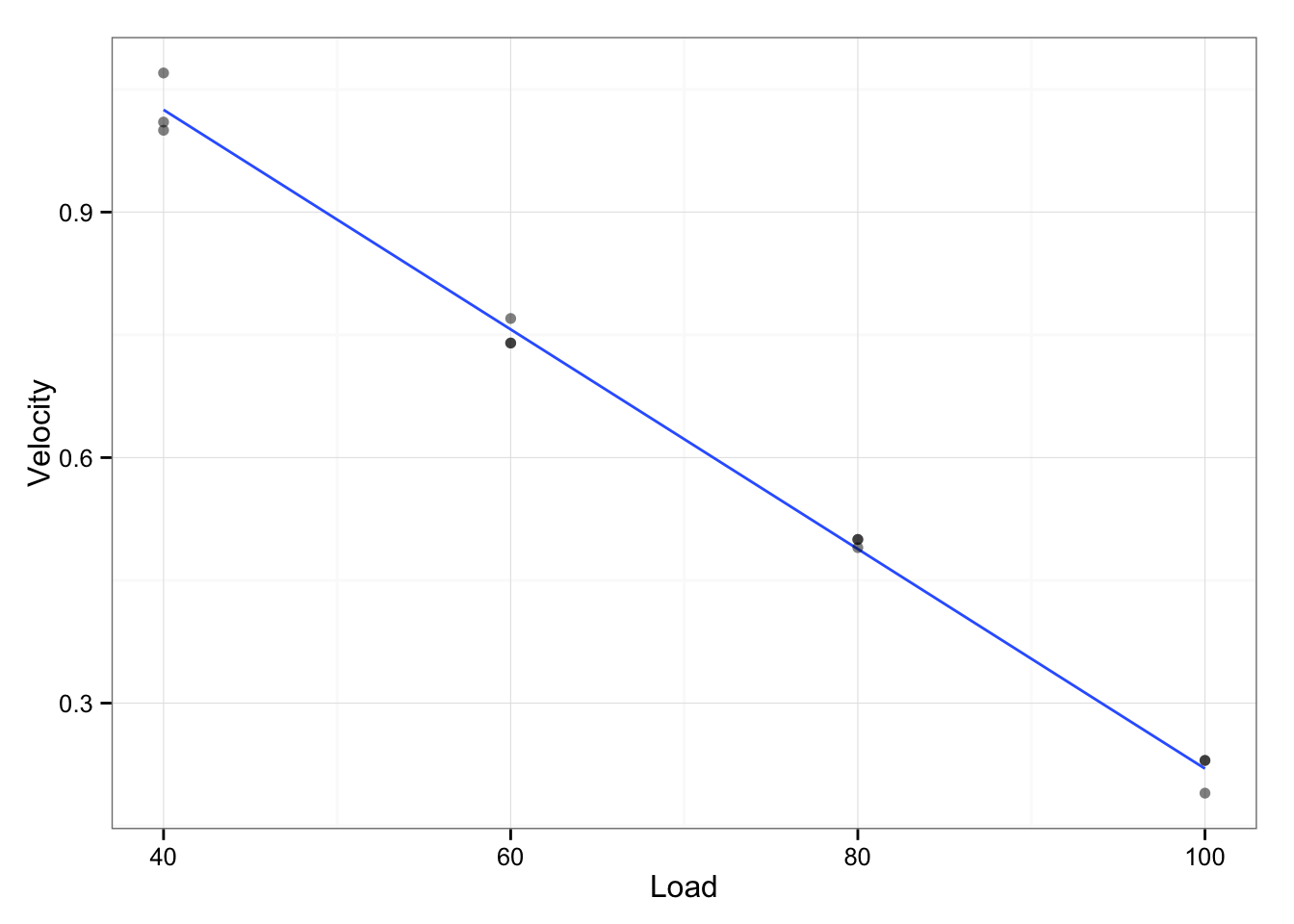
We can create simple Load-Velocity linear model, but what we are interested into are residuals (how much each point differs from model – in this case LV line). We will use residual standard error (note: I will use RMSE – root mean square error)
LV.model <- lm(Velocity ~ Load, data = VBT.1RM.data)
LV.model.residuals <- residuals(LV.model)

residual.SE <- sqrt(sum(LV.model.residuals ^ 2) / length(LV.model.residuals))
This residual standard error (which is equal to 0.02 m/s) could be considered noise. We can use this noise to estimate smallest change in velocity that we can consider real (using 90% confidence, and assuming normal distribution of residuals)
smallest.velocity.change <- qnorm(0.95, sd = residual.SE)
smallest.velocity.change
## [1] 0.03351943Taking smallest velocity change (in this case 0.034 m/s), what is the minimal detectable change in load [kg]?
smallest.load.change <- abs(smallest.velocity.change / coef(LV.model)[2]) # Divide by Load-Velocity slope
smallest.load.change
## Load
## 2.498342The minimal detectable change in load is 2.498 [kg]. This seems very precise.
Now when we know minimal detectable change in velocity and load we should compare it to other smallest meaningful changes in either velocity of load.
First approach wold be to compare it to SWC (smallest wortwhile change) in 1RM which is usually taken as 0.2 x between individual SD. This would tell us if velocity estimates could be used to detect practically significant changes in 1RM.
Second approach would be to compare it to individual practical change in load, and in my opinion that can be change from 4- to 5-RM or any other combo (2- to 3-RM and so forth).
I will use my recent tests with 85% and 70% 1RM (published HERE) as an example.
| Max.Reps | Load | |
|---|---|---|
| 1 | 1.00 | 117.50 |
| 2 | 5.00 | 100.00 |
| 3 | 11.00 | 82.50 |
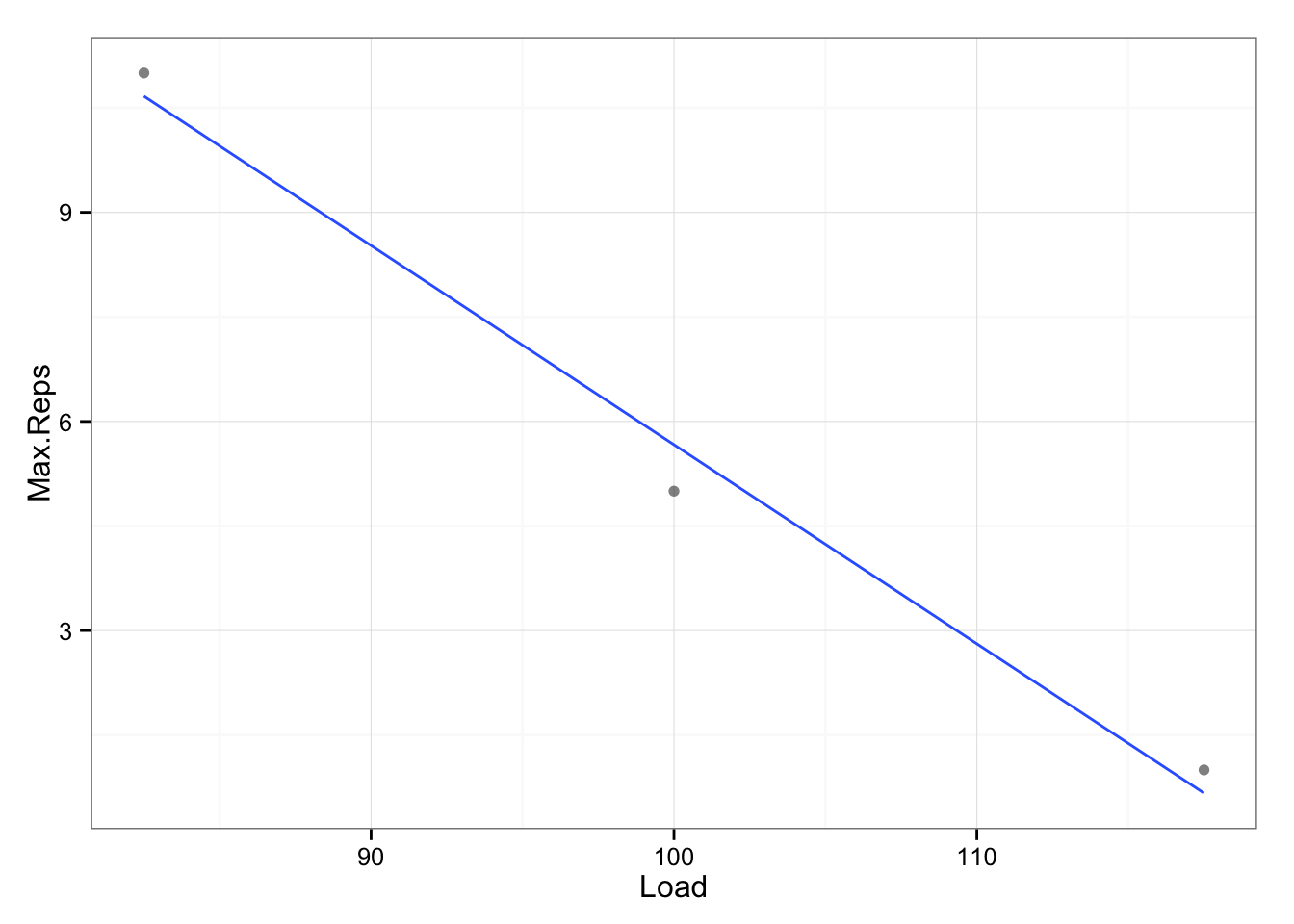
We can again use linear model to create relationship between max reps and load.
max.reps.model <- lm(Load ~ Max.Reps, reps.to.failure.test)
coef(max.reps.model)
## (Intercept) Max.Reps
## 119.572368 -3.453947Since this is linear model, we can use the Max.Reps coeficient (in this case -3.454 [kg]) as signal, which means that for each extra rep, load used must drop by -3.454 [kg].
In this case our noise is smaller than signal. In other words, within-subject variability in velocity is lower that velocity associated with change in N-RM (rep max load).
smallest.load.change / coef(max.reps.model)[2]## Load
## -0.7233296What this means is that we can use velocity to gauge rep-max load.
Third approach involves using “theoretical” relationship between exertion (reps left in the tank) and velocity. I have used data from the same source (click HERE)) as an example
| Reps.left | RM.70.Percent | RM.85.Percent | |
|---|---|---|---|
| 1 | 0 | 0.13 | 0.16 |
| 2 | 1 | 0.24 | 0.24 |
| 3 | 2 | 0.25 | 0.28 |
| 4 | 3 | 0.33 | 0.33 |
| 5 | 4 | 0.36 | 0.39 |
| 6 | 5 | 0.37 | |
| 7 | 6 | 0.41 | |
| 8 | 7 | 0.48 | |
| 9 | 8 | 0.48 | |
| 10 | 9 | 0.51 | |
| 11 | 10 | 0.58 |
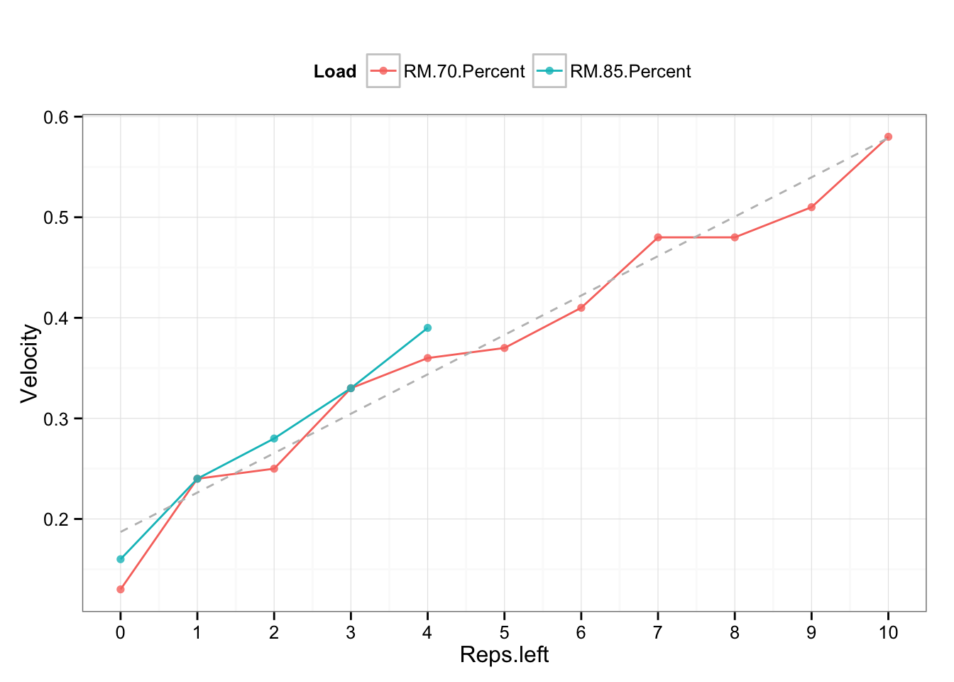
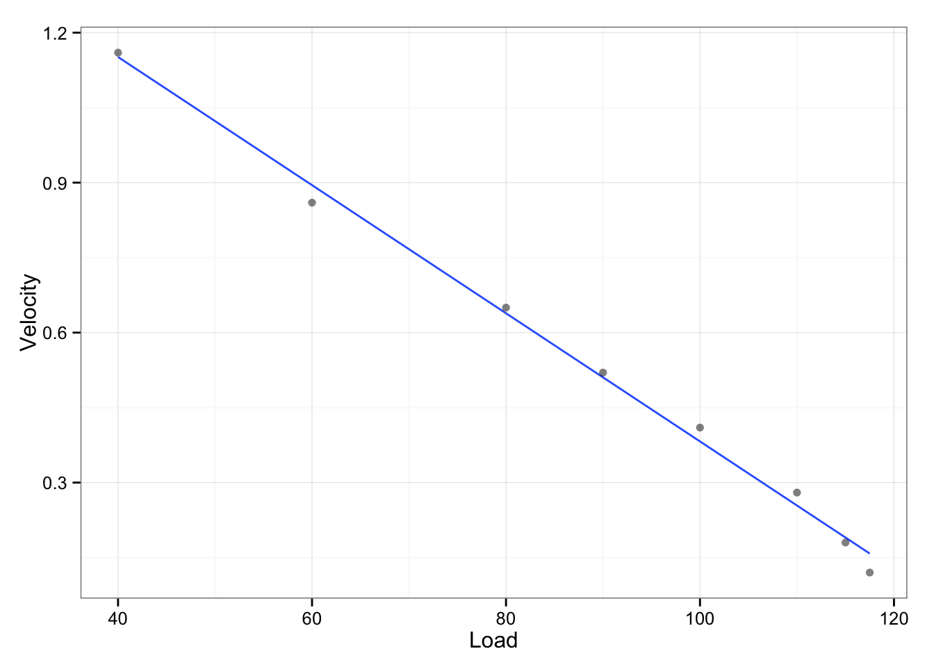
The idea behind load-exertion profile is that velocity associated with reps-left-in-the-tank regardles of the load used is the same (or similar). The extension of this model is that 1RM velocity should be same/similar to 0-reps-left, 2RM should be the same/similar to 1-rep-left and so forth. Let’s check that theory by comparing velocities from from two models and performing t-test. To do that I would need to use 1RM test data from the same data set (since the one used to calculate noise is older, but included multiple sets at given intensity). See the newer test in the table and graph below.
| Set.. | Load | Velocity | |
|---|---|---|---|
| 1 | 1 | 40.00 | 1.16 |
| 2 | 2 | 60.00 | 0.86 |
| 3 | 3 | 80.00 | 0.65 |
| 4 | 4 | 90.00 | 0.52 |
| 5 | 5 | 100.00 | 0.41 |
| 6 | 6 | 110.00 | 0.28 |
| 7 | 7 | 115.00 | 0.18 |
| 8 | 8 | 117.50 | 0.12 |
# Convert to percentages
reps.to.failure.test$Load <- reps.to.failure.test$Load / max(reps.to.failure.test$Load)
max.test.data$Load <- max.test.data$Load / max(max.test.data$Load)

max.reps.model <- lm(Load ~ Max.Reps, reps.to.failure.test)

# Create max reps table
max.reps.table <- predict(max.reps.model, newdata = data.frame(Max.Reps = 1:10))| Max.Reps | Percent.1RM | |
|---|---|---|
| 1 | 1 | 99.00 |
| 2 | 2 | 96.00 |
| 3 | 3 | 93.00 |
| 4 | 4 | 90.00 |
| 5 | 5 | 87.00 |
| 6 | 6 | 84.00 |
| 7 | 7 | 81.00 |
| 8 | 8 | 78.00 |
| 9 | 9 | 75.00 |
| 10 | 10 | 72.00 |
load.velocity.model <- lm(Velocity ~ Load, max.test.data)

# Create velocity-nRM table (velocity associated with nRM)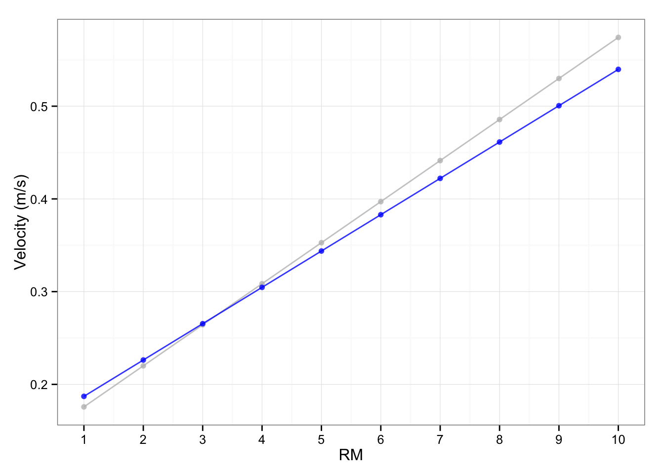
nRM.velocity.table <- predict(load.velocity.model, newdata = data.frame(Load = max.reps.table))| Max.Reps | Velocity | |
|---|---|---|
| 1 | 1 | 0.18 |
| 2 | 2 | 0.22 |
| 3 | 3 | 0.26 |
| 4 | 4 | 0.31 |
| 5 | 5 | 0.35 |
| 6 | 6 | 0.40 |
| 7 | 7 | 0.44 |
| 8 | 8 | 0.49 |
| 9 | 9 | 0.53 |
| 10 | 10 | 0.57 |
# Update Velocity-Exertion profile
exertion.velocity.data$Reps.left <- exertion.velocity.data$Reps.left + 1

exertion.velocity.model <- lm(Velocity ~ Reps.left, exertion.velocity.data)
exertion.velocity.table <- predict(exertion.velocity.model, newdata = data.frame(Reps.left = 1:10))| Max.Reps | Velocity | |
|---|---|---|
| 1 | 1 | 0.19 |
| 2 | 2 | 0.23 |
| 3 | 3 | 0.27 |
| 4 | 4 | 0.30 |
| 5 | 5 | 0.34 |
| 6 | 6 | 0.38 |
| 7 | 7 | 0.42 |
| 8 | 8 | 0.46 |
| 9 | 9 | 0.50 |
| 10 | 10 | 0.54 |
Now let’s perform t-test on two profiles (N-RM-velocity and Exertion-Velocity)
t.test(nRM.velocity.table, exertion.velocity.table)##
## Welch Two Sample t-test
##
## data: nRM.velocity.table and exertion.velocity.table
## t = 0.204, df = 17.738, p-value = 0.8407
## alternative hypothesis: true difference in means is not equal to 0
## 95 percent confidence interval:
## -0.1074942 0.1305838
## sample estimates:
## mean of x mean of y
## 0.3749361 0.3633913As can be seen the difference is not statistically significant (p = 0.8407, ES = -0.09)
Seems like this can be useful model, but it needs more confirmation both in research and real life. In our Exertion-velocity model, change in exertion level yield the following change in velocity:
round(coef(exertion.velocity.model)[2], 3)## Reps.left
## 0.039And our smallest velocity change is 0.034 which is 86%. This means that within-individual variability is less than velocity change associated with change in exertion level. In other words, according tho this data (N = 1) velocity could be used for exertion programming and monitoring.
In all of our cases the noise is less than the signal.
Hopefully this workbook provided some potential ideas for further research on VBT.


Responses