Sprint Profiling – Common Problems and Solutions Part 3

Previous Part:

Sprint Profiling – Common Problems and Solutions Part 2

Timing-gates / photocells or the analysis of the distance-time trace

In this installment of the article series, we will discuss the use of the distance-time trace from the timing-gates (i.e., split times), as well as velocity-acceleration traces from GPS or LPS system. You might be wondering why do we need to discuss distance-time trace since we have already discussed the time-distance trace in the previous installment? There are few rationale for this.

The first rationale is statistical. When we measure with the tether device, or laser, the independent variable is time, while the distance is dependent variable. As we have already explained in the previous installment), this is modeled (or mapped-out) using Equation 1. This is statistically correct way to represent the model given the data.

\[
d(t) = MSS \cdot \left(t + TAU \cdot e^{-\frac{t}{TAU}}\right) – MSS \cdot TAU
\tag{1}\]

When it comes to photo-cells or timing gates, our gates are positioned at given distance, while the time is tracked. In plain English, we have flipped the variables: now the distance in independent variable, while the time to reach the gate (i.e., split time) is dependent variable. Thus we need to use Equation 2, since this is statistically correct model definition given our observed data. Funny enough, all research papers thus far have used Equation 1 to estimate short sprint parameters, until we have pointed to this issues and provided the correct statistical model definition (Vescovi and Jovanović 2021a).

\[
t(d) = TAU \cdot W\left(-e^{\frac{-d}{MSS \cdot TAU}} – 1\right) + \frac{d}{MSS} + TAU
\tag{2}\]

Since we will be referring to this equation all the time in this installment of the article series, particularly for the model definition purposes, I will call it the “time at distance” function (Equation 3). As in the previous installment, this will increase the readability and provide less error when writing the complex equations. Please note that I have used \(\frac{MSS}{MAC}\) as \(TAU\).

\[
time \; at \; dist(d, MSS, MAC) = \frac{MSS}{MAC} \cdot W\left(-e^{\frac{-d}{MSS \cdot \frac{MSS}{MAC}}} – 1\right) + \frac{d}{MSS} + \frac{MSS}{MAC}
\tag{3}\]

The second rationale for utilizing distance-time trace involves specific issues with the timing gates, and these will be discussed next. We will start with almost-perfect measurement setting, and why we cannot achieve this in practice (i.e., real life), and follow with more practical settings, their issues, and potential solutions.

Figure 1 depicts quasi-ideal scenario where the two measurement methods (laser/radar gun and photo-cells) are aligned with the actual sprint (remember the distinction between measurement and sprint scales in first installment of this series LINK). This is in theory the perfect measurement setting we strive to achieve

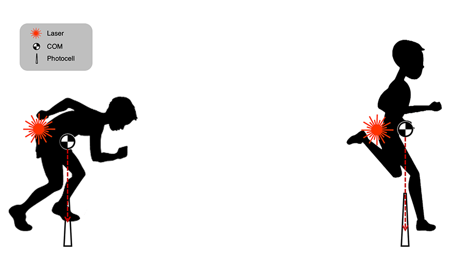
Figure 1: Quasi-ideal alignement between sprint center-of-mass (COM) and measurement using timing gates and laser gun. See text for explanation

Ideally, we would want to measure the instantaneous position (as well as velocity) of the center-of-mass (COM). This can be achieved with 3D cameras and correct body model. Unfortunately, most of us do not have access to such an equipment. The closest we can get to this scenario practically, is by using laser/radar run. But in this case, we do not measure position/velocity of the COM, but of the body location at which the laser/radar is pointing at. Since these are usually positioned around 1-meter from the ground, the body position will be different at the start (particularly when utilizing block or three-point start) versus at the sprint finish. Due to the torso thickness and changes in COM position due to body parts moving, there will be systematic as well as variable difference between laser/radar point position and COM position. For this reason, I have termed the setting depicted in Figure 1 quasi-ideal.

Besides laser/radar gun, Figure 1 assumes that timing gates/photocells are also triggered by the COM and not by the torso or limbs. Initial timing gate, at least in theory, should be triggered by the change in COM position, and the athlete should not have any pre-sprint movements (e.g., body shifts, or arm movements) (see the left side of the Figure 1). This is needed for the timing start to be perfectly aligned with the actual sprint start. Closest to this would be that the athlete starts within the beam of the timing gate. As far as I am aware, there are still no such methods implemented in the initiation of the timing, but some vendors are developing something along those lines. There are foot or hand pods that can be used instead – for example there can be a switch behind the rear foot with the standing start.

Besides the initial gate, photocell beams will be triggered by the torso or limbs passing by, rather than COM. Thus the right side of the Figure 1 is also impossible to achieve in practice.

Figure 2 depicts more realistic alignment of both the initial timing gate and the end (or intermediate) timing gate(s). In this scenario, the start line is aligned with the beam of the photocell (i.e., in the case of the standing start, the top of the foot is positioned on the line, or on the line edge, which can be 2.5 – 5cm behind the beam). This will result in COM being behind the start line, as well as the laser/radar gun point, which will be further back. The problem with this setup is that now the limb movements (either during the setup, or before a start) will trigger the timing of the photocell. Also, the later photocells (i.e., right side of the Figure 2) can also be triggered by the limb motion, rather than the COM or torso, creating random measurement error, which decrease the sensitivity of the measurement to capture true performance. There are few solutions to this – (i) some vendors have photocells with double beams, reducing the likelihood of triggering the system with limbs, and (ii) using microprocessor that detects the longest time crossing of the beam, assuming the longest crossing is the torso (Bond, Willaert, and Noonan 2017; Bond et al. 2017). None of these completely remove the random error.

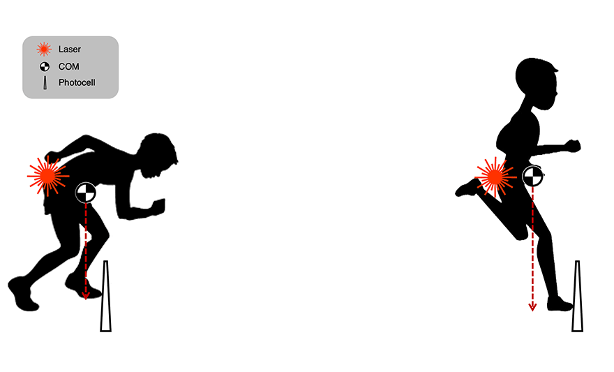
Figure 2: More realistic alignement between sprint center-of-mass (COM) and measurement using timing gates and laser gun. See text for explanation

To solve the issues of the premature triggering of the initial timing gate, athletes are often moved further back away from the initial photocell beam (Figure 3). This moves the COM further back, resulting in flying start. We will explore the potential issues with this technique as well as potential solutions in the next sections.

How do we achieve alignment between laser/radar gun and timing gates? In short – we can’t, at least not perfect. The laser/radar beam will always be behind the COM, and the photocell beam will always be in front. Both will suffer from random error as well as fixed error (i.e., constant difference) just explained. The random error with the laser/radar gun will come from changes in the COM position and body posture, while with photocells will come with limb triggering. It thus makes little sense to compare the split times between the systems. There are some solution that can reduce the magnitude of the systematic difference by triggering both the laser/radar and initial timing gate using the floor trigger or pad, but the distance will always be slightly different.

And here comes the Acceleration-Velocity Profile (AVP) to help. Rather than comparing split times, we can compare the estimated \(MAC\) and \(MSS\) parameters. And this is exactly the topic of my PhD thesis: comparing the AVP estimates from the laser gun vs the timing gates [Jovanović (2023); Vescovi and Jovanović (2021a); third one in in the submission process].

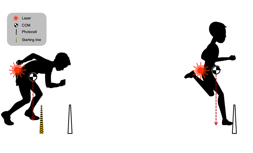
Figure 3: To avoid cutting the beam of the timing gate (i.e., photocell) prematurely, athlete starts behind-the-line with the COM more misaligned with the measurements, resulting in the flying start. See text for explanation

Now that we have covered the measurement scale misalignment with the actual sprint scale, let us discuss some specific biases that can arise from distance-time trace, assuming perfect alignment with the COM position/velocity.

To create sprint traces, we will use the create_sprint_trace() function from the {shorts} package with known true values of \(MSS\), which is set to 8 \(ms^{-1}\), and \(MAC\), which is set to 6 \(ms^{-2}\). Besides creating simulation with sprint scale completely overlapping with measurement scale (i.e., \(t=0s\) and \(d=0m\)), we will create few more problematic issues involving time shift, distance shift, flying sprint distance, and combination. We will discuss each of these and how to address them.

Normal trace