Review and Retrospective – Part 2

In case you missed the previous parts of this article series you can find them here:

1. Introduction
2. Agile Periodization and Philosophy of Training
3. Exercises – Part 1 | Part 2
4. Prescription – Part 1 | Part 2 | Part 3
5. Planning – Part 1 | Part 2 | Part 3 | Part 4 | Part 5 | Part 6
6. Review and Retrospective – Part 1

Dose – Response models

Besides simple descriptive modeling outlined with the previous models, we can use data collected to gain some insights into the dose – response relationships. The gross categories of data analysis involve (1) description, (2) prediction and (3) causal inference ¹ (Hernán, Hsu & Healy, 2019). Description can be quite simple, and so far we have utilized this category the most. For example, average relative intensity (aRI), number of lifts and other dose metrics represent simple descriptors. Prediction on the other hand aims to predict outcome from supplied predictor variables, while avoiding the pitfalls of overfit and underfit. For example, if I perform 50 NL in the squat today, what effect can I expect three days later on my estimated 1RM in the back squat. Causal inference aims to understand causation behind the variables. For example, understanding effects of NL in the squat and deadlift on squat 1RM, as well as their interaction. But to make causal claims, predictive analysis is not enough, so we either employ controlled randomized experiments or use observational studies with high scrutiny and previous domain knowledge ² (Angrist & Pischke, 2015; Pearl, Glymour & Jewell, 2016; Hernán, 2017; Pearl & Mackenzie, 2018; Hernán & Robins, 2019; Hernán, Hsu & Healy, 2019; Pearl, 2019).

I will illustrate one predictive approach that can serve as an additional source of information for the review and retrospective (see Figure 2.13). We have ten athletes, performing either Total, Upper or Lower workouts in random fashion, using easy, medium and hard workloads over 90 days. Upper body NL and Lower Body NL is tracked. Estimated 1RM (est1RM) in the bench press is used as a target variable. Measurement error for est1RM is assumed to be normally distributed with SD of 0.5kg.

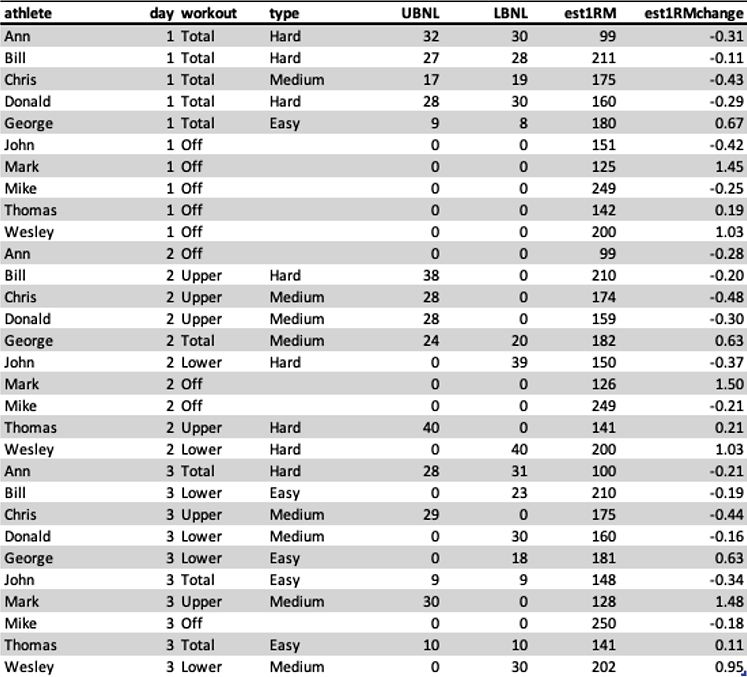
Table 6.1. Example data collected for five athletes. LBNL represents lower body number of lifts, and UBNL represent upper body number of lifts for a day

You probably noticed that each athlete has different starting 1RM (day 1). Estimated 1RM change (est1RMchange) is what is actually modeled here (i.e., target variable), since we are interested in effect on 1RM (e.g., how much it changes), rather than raw value of 1RM. Particularly since out athlete have different 1RM values.

As any other model, this is highly subjective, since it is a subjective decision of which variable goes inside the model, and how the metrics should be engineered for a prediction task. Labs coats can cry ‘objectivity’ all day long, but every single model is subjective. We just want to make sure this subjective model can give useful predictions, can be falsifiable, and can generate new ideas and insights (Gelman & Hennig, 2017; Amrhein, Trafimow & Greenland, 2019). These should be then evaluated together with other sources of evidence (see Figure 2.13 and the discussion on evidence-based practices)

Figure 6.11 depicts this data, but to put everything on the same scale, pooled ³ UBNL, LBNL and est1RM has been scaled from 0 to 1.

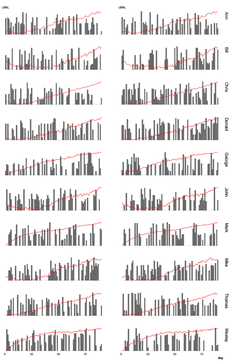
Figure 6.11. Upper and lower body NL across 90 days with est1RM (red line). Numbers are scaled from 0 to 1.

Figure 6.12 depicts raw 1RM for five athletes as well as change in 1RM from day to day (which can be considered first derivative of 1RM).

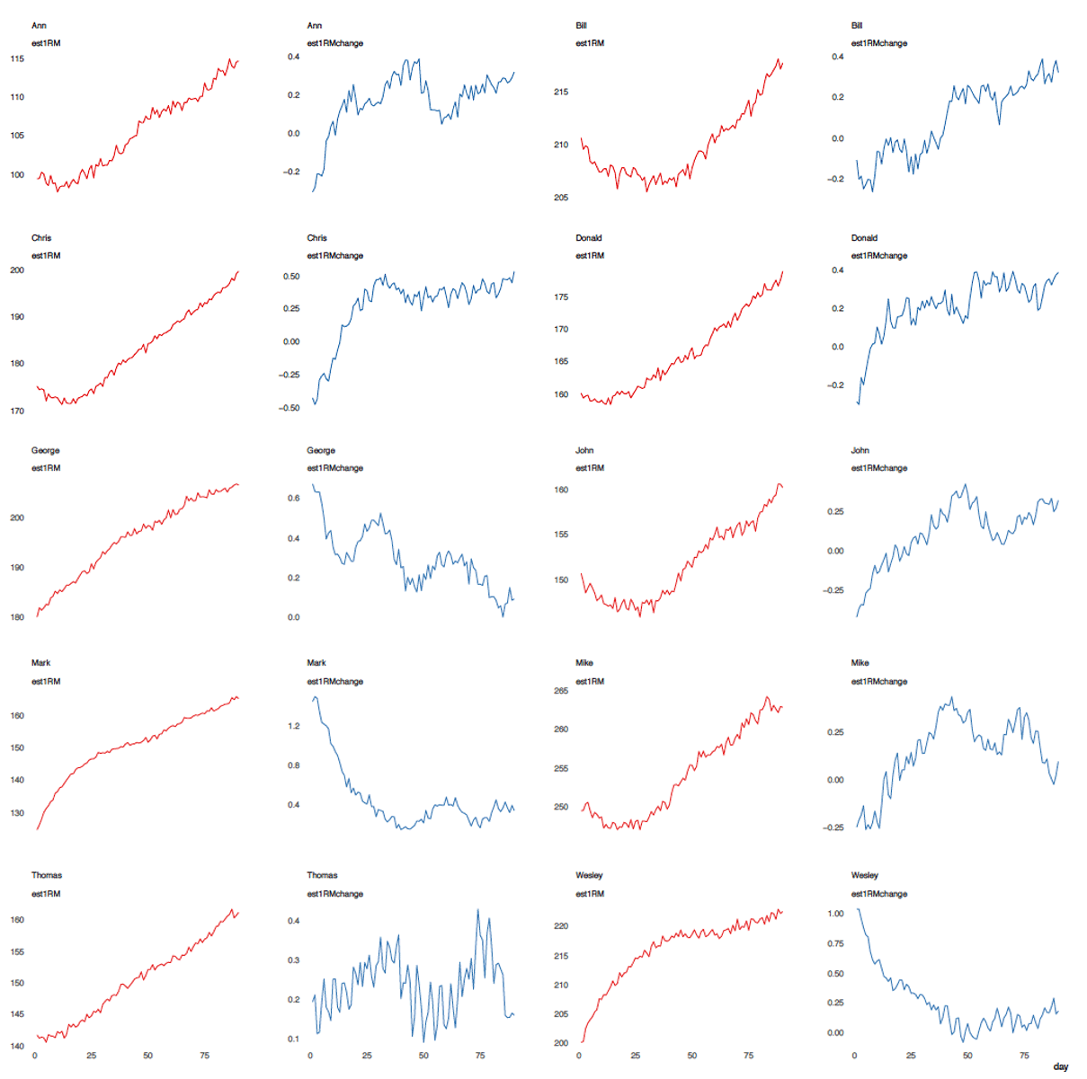
Figure 6.12. Raw 1RM and change in 1RM across 90 days

Table 6.2 represents overly simplistic descriptive analysis of the above 90 training days.

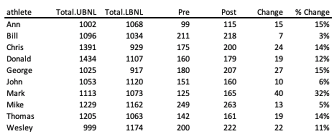
Table 6.2. Aggregated effects over 90 days

Table 6.2 can then be used in linear regression to estimate effects of NL on Change or % Change in 1RM. If we had Control group, that either did nothing, or some standard protocol, and the Intervention group that did something novel, we could estimate causal effects on intervention on Change or % Change. If the variables in the intervention group differ (e.g. NL), we could control for that by using ANCOVA rather than ANOVA (please note that both are extension of the linear regression model). The point is that, although it sounds “objective” and “evidence based”, this approach is also subjective, since we decided to represent complex world (Large World) with simple pre- and post- aggregates (Small World). In this particular example, we can see that there are many nuances in the response variable as well as with the dose variables (see figures 6.11 and 6.12) which cannot be picked­-up with simple aggregated table (Table 6.2).

In the following paragraphs, I will predict daily 1RM, rather than the aggregate pre- and post- scores (e.g., by using Table 6.2). But without the control group, we are unable to claim any causal effects, since the effects could be due to third variables (e.g. growing up, using steroids, nutrition) that we didn’t control or account for. To do this, I will use random forest model, and feature engineering using acute and chronic EMA, as well as lag variables from 1 to 10 days (Jovanovic, 2017a,b, 2018a,b; Kuhn & Johnson, 2018). This is again just a subjective choice. To evaluate performance of the model and to select the best tuning parameter, 5-folds cross validation is used. The only athlete that is unseen by the model, and serves as a test data is Wesley.

Figure 6.13 depicts true 1RM and predicted 1RM using the model. Since Wesley serves as test data, it can be easily seen how biased the model is for him. It seems that the model is fine for predicting general patterns.

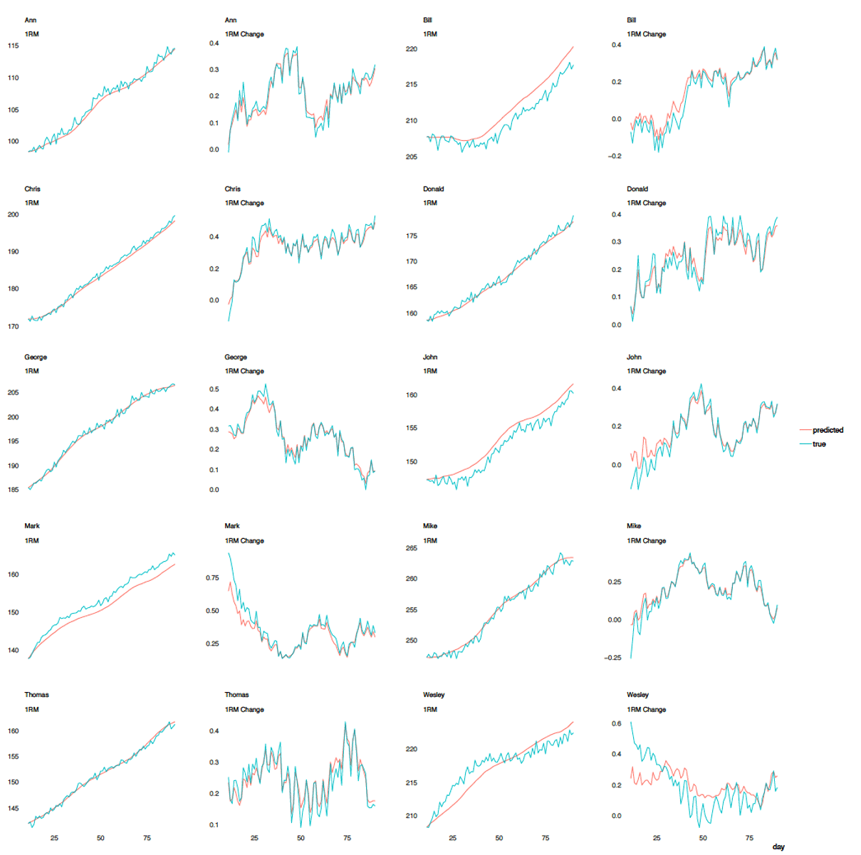
Figure 6.13. True and predicted daily 1RMs

If we conclude that the above model has predictive validity, we can use the same model to predict response in various scenarios. One just needs to watch not to extrapolate and use combinations of variables that are not present in the training data (Kuhn & Johnson, 2018). This topic is beyond the scope of this manual.

Since random forrest is a black box model, certain techniques can be used to get a glimpse on how the model behaves when probed. For example, we might be interested in variable importance, or in other words, figuring out on which variable prediction depends the most (Molnar, Bischl & Casalicchio, 2018; Molnar, 2018; Kuhn & Johnson, 2018).This is done by permutating single variable and estimating the prediction error. The variable whose permutation creates the biggest prediction error is the most important variable. Figure 6.14 contains the top 10 most important variables for this model given the training data.