Predicting Non-Contact Hamstring Injuries by Using Training Load Data and Machine Learning Models

Introduction

In running-based team sports (e.g. soccer, handball, basketball, rugby), non-contact hamstring injuries remain one of the major reasons players spend time on the sideline. Losing players for multiple weeks due to the hamstring (or any other non-contact) injury can cost clubs not only winning games and championships but can also be a huge financial loss. Estimating the likelihood of non-contact hamstring injuries and intervening with appropriate actions on those predictions is the “holy grail” of applied sports science.

The aim of the current paper is twofold. The first aim is to estimate the predictive performance of multiple non-contact hamstring injury prediction models, by using day-to-day collected training load data. Second aim is to follow up on the data preparation method outlined by the author in the previous paper,¹ with predictive modelling on the real data set. The data set used in the current paper was given to the author, for the purpose of analysis by a sports organization that prefers to remain anonymous. The name of the athletes, days, training load metrics, and any other data is made anonymous by the author. The author cannot claim the validity of the data set used in the current paper, due to the fact that the author has not been involved in the data collection, cleaning, and storing of the data. Having said this, the results of the current paper should be viewed highly skeptically and with a high level of concern. The purpose of the current paper is thus educational and speculative, with special emphasis on presenting a potential approach in predictive modeling of day-to-day training load data, with the aim of predicting non-contact hamstring injuries.

Methods

Athletes

This study was conducted during the preparatory and competition periods of Season 1 and Season 2, in anonymous sports club for N=52 athletes, over 600 days in total (Season 1: N=45 for 307 days and Season 2: N=45 for 293 days, where N=38 athletes were present in both seasons) (see Figure 1).

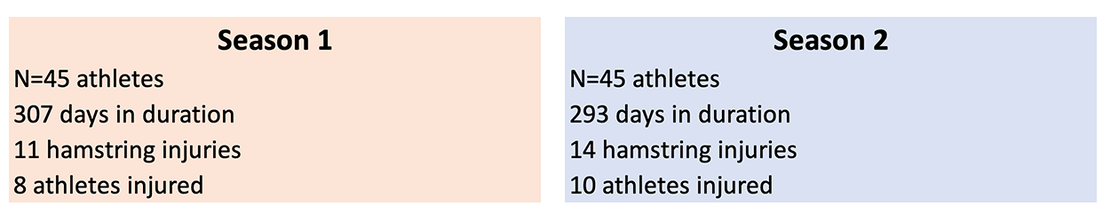
Figure 1. Characteristics of Season 1 and Season 2

During this time period, 25 non-contact hamstring injuries occurred (11 in Season 1 and 14 in Season 2) for 17 athletes (8 athletes in Season 1 and 10 athletes in Season 2 suffered non-contact hamstring injuries). (see Table 1)

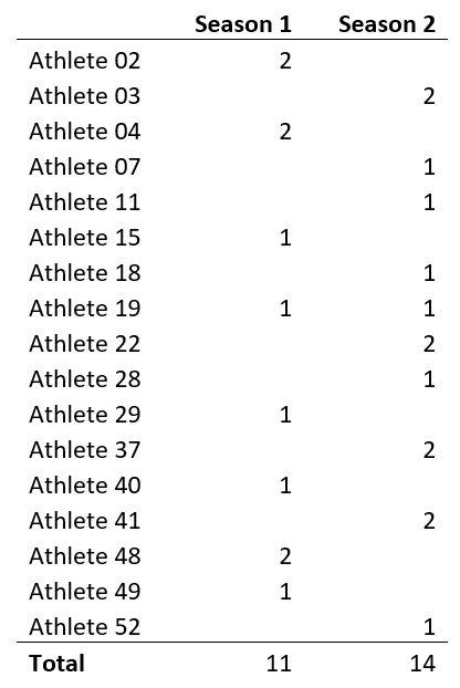
Table 1. Athletes that suffered overuse hamstring injuries during Season 1 and Season 2

Design

This study involved a day-to-day collection of training load and non-contact hamstring injury data (collected over Season 1 and Season 2 competition seasons including matches); (b) the modeling of training load with injury, with the aim of predicting the occurrence of a non-contact hamstring injury. In order to estimate the predictive performance of multiple classification machine learning models, the collected data was split into two partitions: (a) training data set and (b) testing data set 2. Training data set was used to train the models, while testing data set was used to estimate predictive performance on unseen data. Although I suggested splitting the data into training and testing data sets by using seasons ² (e.g. Season 1 as training data set, and Season 2 as testing data set), due to the small number of injury occurrences, the data was split by using athletes instead. Data from both seasons for athletes “Athlete 02”, “Athlete 03”, “Athlete 40”, and “Athlete 52” was used as testing data set. Splitting the data by using this method, rather than seasons, has achieved multiple goals: (1) more injury occurrences are used to train the models, (2) potentially different loading patterns from two seasons are taken into account, and (3) models are evaluated on the unseen athletes, which represent an ecologically valid way to evaluate the model.

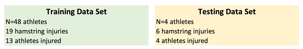
Figure 2. Characteristics of training and testing data sets

Methodology

Training load

Session training load was represented by using three training load metrics. The name and the origin of training load metrics remain anonymous. Training load metrics were mostly captured for all training sessions, which included skill sessions and matches, resistance training sessions, recovery sessions, off-legs conditioning sessions, as well as rehab sessions. Due to the data acquisition nature, some training load metrics were not acquired on certain types of training sessions. Thus, with reported and used three training load metrics in this study, “total” training load was not represented in a satisficing manner.

Training load data was represented by using day-to-day instance for every athlete, and in case of multiple training sessions per day, training load data was summed together to get the daily training load. Training load for non-training days was zero, for all three metrics. In the cases of missing data, the data was imputed using MICE procedure ^{3 4}.

Injury definition

For the purposes of this study, an injury was defined as any non-contact, soft-tissue hamstring injury sustained by an athlete, during a training session or match, that prevented the player from completing the entire training session or match. Other types and locations of injuries were collected over the duration of this study, but were not taken into analysis and were assumed to have no effect on the likelihood of suffering a non-contact hamstring injury. Since the author was not involved in injury data collection, the validity of the injury data used in the current study cannot be claimed.

Data preparation (Feature engineering)

Data collected was organized in day-athlete instances (one row of day data for each athlete), and the injury occurrence was tagged on a given day as “Injured” versus “Non.Injured” for all other days (see Table 2).

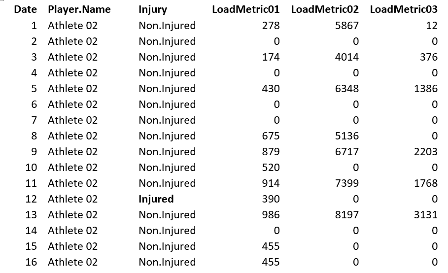
Table 2. Data organization into day-athlete instances

In order to be used in predictive model, new features have been engineered. Data preparation for injury prediction utilized in this study is outlined in the paper by the author, ¹ with a few additions listed below. Every engineered feature was rounded to the closest two decimals.

Acute and Chronic Rolling averages
For each of the three training load metrics, Acute and Chronic metrics were calculated by using the exponential rolling averages. The alpha parameter was calculated by using 2 / (Days + 1) equation, whereas Acute training load was calculated by using 7 days exponential rolling average (alpha=0.25), and Chronic was calculated by using 28 days rolling average (alpha=0.069).

Acute to Chronic Ratio and Difference
In order to normalize Acute and Chronic training load features, additional ratio (Acute to Chronic Workload Ratio (ACWR)) and difference (Acute to Chronic Workload Difference (ACWD)) between the two had been calculated and included in the model.

Rolling Max and Rolling Mean
Two additional features have been calculated for Acute, Chronic, ACWR and ACWD features and they included the last 7 days rolling maximum and rolling mean.
After the above-explained feature engineering procedures, each daily training load metric (LoadMetric01, LoadMetric02, and LoadMetric03) has got an extra 12 engineered features, totaling in 36 features (where the original daily training load metrics were removed).

Lag Features
In order to help in modeling effects of training load preceding injury occurrence (i.e. creating a memory in the data set), an additional feature engineering has been applied and it involved creating the additional three lag variables for each of the previously engineered 36 features. This step involved creating 0, 7, 14, and 21 days lag variables, totaling 144 engineered features (see Table 3). In theory, this helps in modeling delayed training load effect on injury likelihood (i.e. training load spike that occurred 2 weeks ago, might affect injury likelihood 2 weeks later).

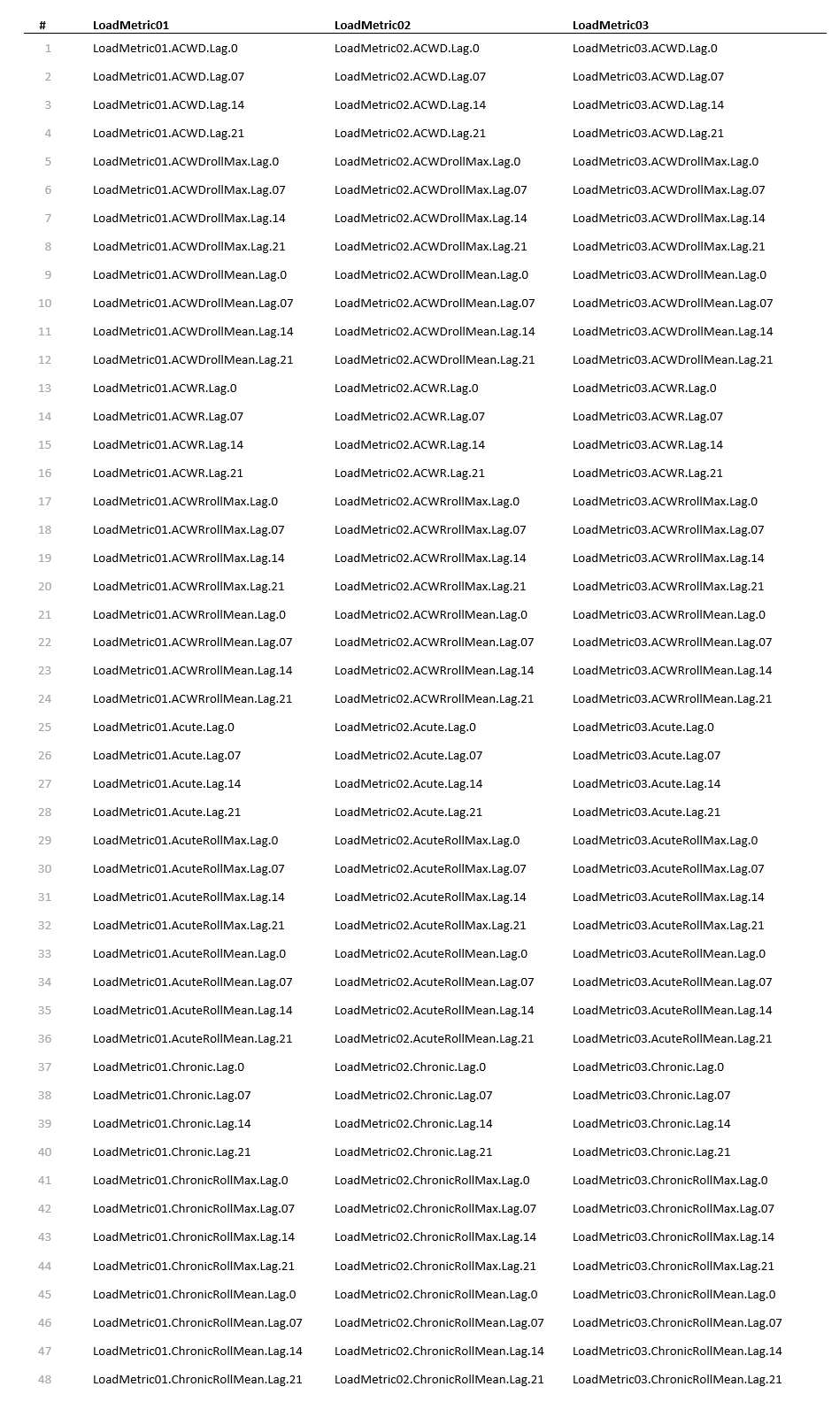
Table 3. Engineered features from the three training load metrics

Injury Lead feature
Non-contact hamstring injury occurrence was tagged only once on the day when it occurred (see Table 2, Injury column). To create early warning signs, as well as to increase the number of injury occurrences in the data set, and help predictive models by creating a potential overlap between the preceding training loads (using the above-explained Lag features) and injury occurrence, the three target features have been created by using 7, 14 and 21 injury lead days (see Table 4).

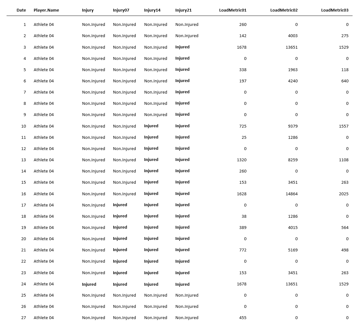
Table 4. Injury Lead features for 7, 14 and 21 days

These three features (Injury07, Injury14, and Injury21) represent target variables in the predictive models. With the data organized this way, machine learning models estimate the likelihood of getting non-contact hamstring injury in 7 or less, 14 or less, and 21 or fewer days. The performance of each machine learning model will be reported for each injury target variable.

Statistical analysis

All analyses have been performed in R statistical language ⁵ by utilizing caret package, ^{6 7} with the following machine learning models: (a) Principal Component Logistic Regression (Logistic Regression), (b) Random Forest ⁸ (2000 trees and 10 tuning parameters), (c) Elastic-Net Regularized Generalized Linear Models ⁹ (GLMNET) (10 tuning parameters), (d) Neural Network ¹⁰ (Neural NET) (maximal number of iterations 2000 with 10 tuning parameters), (d) Support Vector Machine with linear kernel ¹¹ (SVM) (10 tuning parameters). Each machine learning model was trained by using training data set using Injury07, Injury14 and Injury21 as target variables, and estimated predictive performance on testing data set (see Figure 2). For each machine learning model, the best tuning parameter was selected based on a cross-validated predictive performance by using AUC metric ⁷ (Area Under Receiver-Operator Curve).

Cross-validation method

The most valid method to perform cross-validation would be using “leave-one-injured-athlete-out” (LOIAO) (see Figure 3). LOIAO cross-validation involves leaving one injured athlete (who suffered at least one injury in the training data set) and training the model on the rest of the data. AUC as a measure of predictive performance is calculated for the left-out athlete. The process is repeated for all injured athletes in the training data set, and the final model tuning parameter was selected based on the highest averaged cross-validated AUC metric.

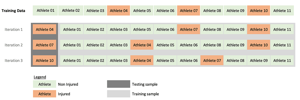
Figure 3. Cross-validation by using “leave-one-injured-athlete-out” (LOIAO)

Unfortunately, LOIAO cross-validation, although ecologically the most valid method to evaluate predictive performance for the problem at hand (since we are interested in how the model predicts on new unseen athletes), was not utilized in the current paper. The main issue with LOIAO cross-validation is a very small number of injury occurrences (since we are predicting on only one athlete) and, thus, unreliable estimation of AUC. For the purposes of the current paper, repeated cross-validation with 3 folds and 10 repeats was utilized.

SMOTE Sampling

A data set is imbalanced if the classification categories are not approximately equally represented. This was the case in both training and testing data sets, since the number of “Injured” instances is less than 3% of the total number of instances in both training and testing data sets, for Injury07, Injury14, and Injury21 target variables.

SMOTE sampling technique uses over-sampling of the misrepresented class (in this case “Injured”), and under-sampling of the overrepresented class (in this case “Non.Injured”), to achieve more balanced samples used in training machine learning models ^{6 7 12}. SMOTE was applied in each cross-validation iteration.

Area Under Curve (AUC)

Predicting “Injured” versus “Non.Injured” instances, represent classification problem in machine learning. For the purposes of this study, AUC metric was used to estimate predictive performance of the machine learning models ^{7 13}. AUC is expressed in arbitrary units, where 1 is perfect prediction and 0.5 is equal to random guess.

Results

Figure 4 depicts training, cross-validated and testing data set predictive performance of all five machine learning models for Injury07, Injury14, and Injury21, as target variables by using the AUC metric. Horizontal error bars represent 95% bootstrap confidence intervals (using 2000 resamples) ¹³.

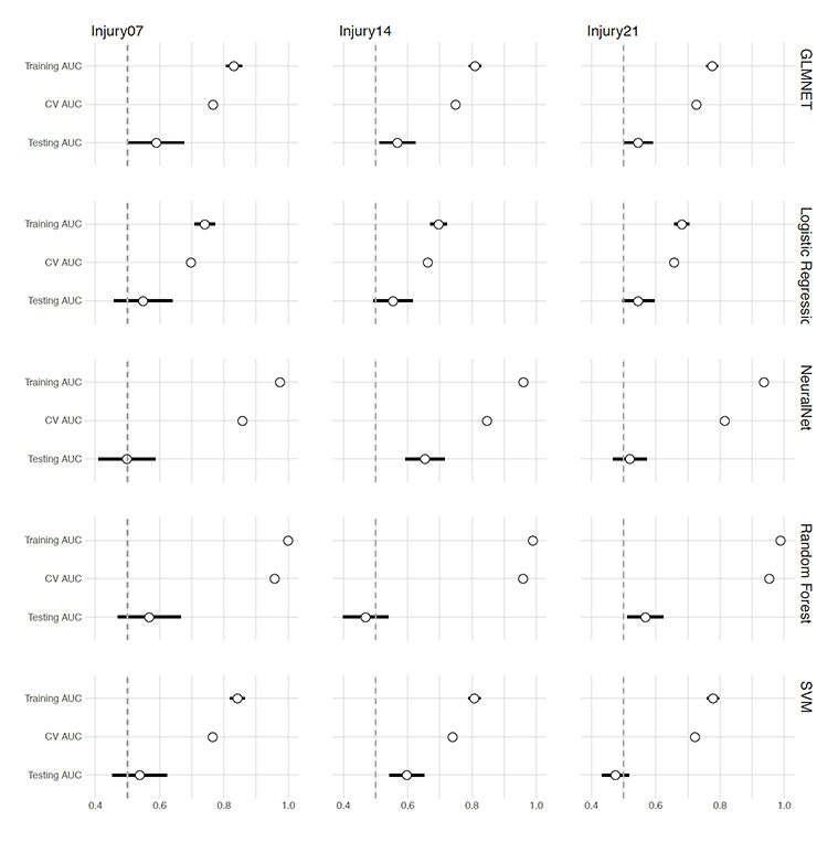
Figure 4. Prediction performance of five machine learning models by using the AUC metric (arbitrary units)

From all of the models, Random Forest had the perfect prediction on training data set for all three target variables (Injury07, Injury14, and Injury 21), but it suffered from overfit ⁷, as can be seen through the poor performance on testing data set. Overall, all models showed poor predictive performance on the testing data set (less than 0.65 AUC, where 0.5 AUC is a ran-dom guess, and 1 AUC is perfect prediction). All models, ROC, and predictions can be found in Supplementary Material.

Discussion

Model performance on training data set can be optimistic and suffer from overfit, or, in other words, model can confuse noise for the signal ⁷. To control for making overfit errors, cross-validation and hold-out (testing) data set are utilized. Figure 5 depicts Random Forest predictions for Injury14 target variable on training data set.

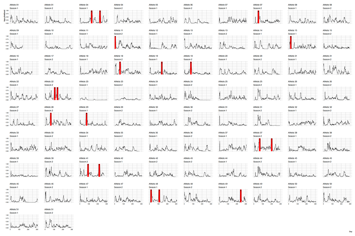
Figure 5. Training data set Random Forest model predictions by using Injury14 as a target variable. Lines represent likelihood of suffering from non-contact hamstring injury in 14 or less days. Red bars represent the actual injury occurrence (with 14 days injury lead).

From simple visual inspection of the graph, it can be seen that prediction is perfect, because the model predicts very high likelihood of injuries in the red bars (red bars represent the actual injury occurrence, with 14 days injury lead). Figure 6 depicts ROC curve for the discussed training data set Random Forest model performance for Injury14 target variable.

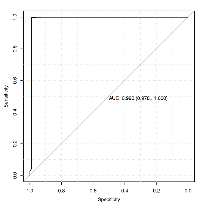
Figure 6. ROC for training data set Random Forest model for Injury14 target variable. AUC is expressed in arbitrary units and 95% bootstrap confidence intervals are reported in the brackets.

From Figure 5 and Figure 6, one can conclude that non-contact hamstring injuries can be perfectly predicted. But when this very same model is evaluated on testing data set (unseen by the model), the predictions (Figure 7) and ROC curve (Figure 8) look much different, ac-tually worse than a random guess (0.47 AUC).

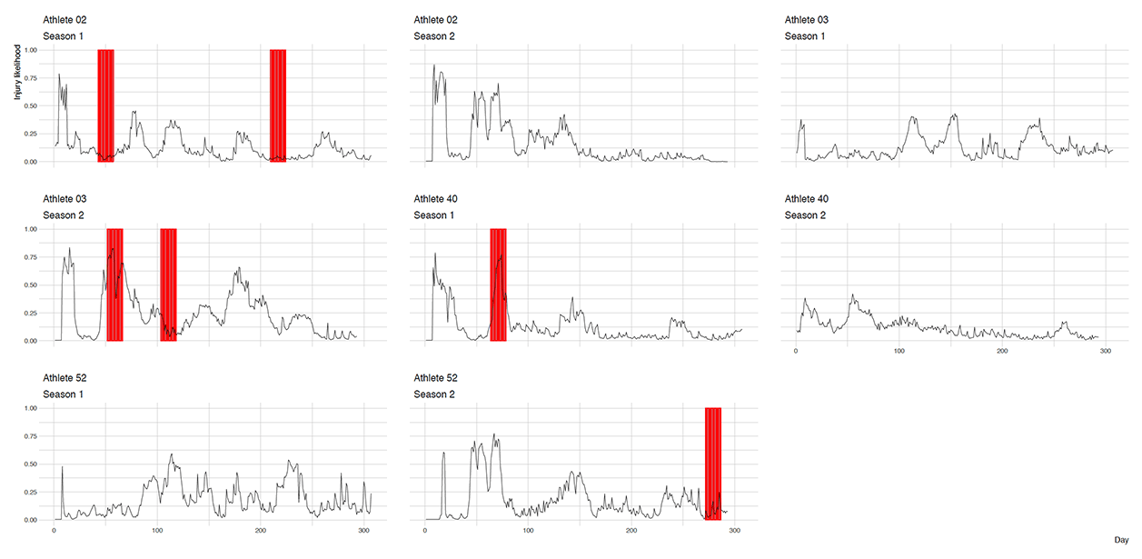
Figure 7. Testing data set Random Forest model predictions by using Injury14 as a target var-iable. Lines represent likelihood of suffering from non-contact hamstring injury in 14 or less days. Red bars represent the actual injury occurrence (with 14 days injury lead).

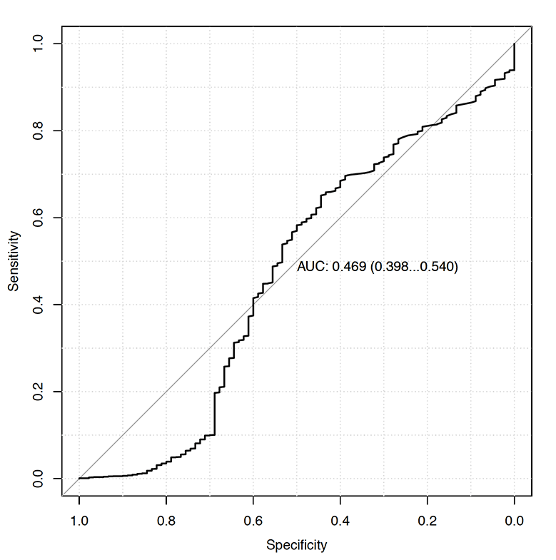
Figure 8. ROC for testing data set Random Forest model for Injury14 target variable. AUC is expressed in arbitrary units and 95% bootstrap confidence intervals are reported in the brackets.

Practical applications

In the current study, by assuming validity of the data analyzed, it can be concluded that the non-contact hamstring injuries could not be predicted by using training load data with features engineered, as described previously. To paraphrase Nassim Taleb, author of Black Swan ¹⁴ and Antifragile ¹⁵ books: “It is far easier to figure out if something is fragile, then to predict the occurrence of an event that may harm it”. Practitioners should hence spend more time and effort in building more robust athletes, than trying to predict injury occurrences ².

Limitations

Representing complex reality with simple models. always include many assumptions and most likely misses out numerous factors ². In the current study, there have been many assumptions and limitations involved in the data representations and modeling:

• Only three training load variables are used, whereas many more could be utilized.
• Assumptions that previous injuries (hamstring or other related ones) don’t affect future non-contact hamstring injuries.
• Assumptions that athlete’s characteristics (age, experience, weight, previous injury), performance testing (i.e. strength levels, aerobic endurance, maximal speed), as well as medical screening (stability and mobility issues and so forth), don’t affect training load effects on injury likelihood.
• Assumptions that athlete’s readiness, wellness, nutritional and emotional status don’t affect training load effects on injury likelihood.
• Assumption that match outcome doesn’t affect emotional response by the athlete, hence, has no effect on training load effects on injury likelihood.
• Assumptions that external conditions, like shoes, surface, weather, time of the day and so forth, don’t affect training load effects on injury likelihood.
• Data collected only for one sports club, over two competitive seasons.

Enlisting all limitations and assumptions (known and unknown) can probably be a paper itself. Collecting more data for a longer period of time (i.e. the whole league for 5-10 years), might bring some insightful information and it could be a fruitful strategy to employ. In machine learning, there is a heuristic “More data beats better algorithms” ¹⁶. Even with such an enterprise, numerous modeling assumptions will be present, and practitioners should look at model predictions as only one source of information or evidence to direct their practices. Other sources of actionable insights should be simple rules of thumb or heuristics (such as those proposed by the author ², coaching intuition, and using multi-model approach ¹⁷. Even if injury prediction models show more promising predictive performance in the future, they don’t sort out intervention and causal problems ²:

• How will intervening on predictions change the outcome and model parameters (author has named this “Minority Report Paradox”, after a famous movie with Tom Cruise), since interventions rely on model parameters “stationarity” assumptions. This brings another issues, on how intervention should be represented in the model itself and how often the model needs to be rebuilt
• How do we go about reporting injury likelihood to athletes themselves? Should they be aware of the injury likelihoods and how is that going to affect the injury likelihood itself (e.g. how will telling athlete that he or she has high likelihood of non-contact hamstring injury in the next 21 days or less, impact his/her performance and emotional state, and how will that affect the actual likelihood itself). This is another example of “Minority Report Paradox”.

Predicting future events is hard, but what is even harder, is acting on these predictions. One potential solution is to look at model predictions as only one source of insights (e.g. “what training load history has to tell us?”) that needs to be put into the correct context (together with intuition and heuristics as other sources of actionable insights), acted upon it with a grain of salt, and frequently re-built with the latest data and intervention information. Together with Nassim Taleb quote, this current paper is best finished with the quote by Abraham Lincoln: “The best way to predict the future is to create it”.

Click here to download the paper in PDF format (printer friendly version)

Supplementary Materials

Accompanying R code, analysis graphs (ROC curves and predictions), as well as raw and prepared training load data are available on GitHub repository:

https://github.com/mladenjovanovic/predicting-hamstring-injuries

Citation and license

Current paper and accompanying code are under MIT license

For citations please use the following:

Jovanovic, M. (2018). Predicting non-contact hamstring injuries by using training load data and machine learning methods. Complementary Training. DOI:10.13140/RG.2.2.20881.68968. URL: www.complementarytraining.com/predicting-hamstring-injuries/

References

1. ¹ Jovanović M. Data Preparation for Injury Prediction. sportperfsci.com. 2018
2. ² Jovanović M. Uncertainty, heuristics and injury prediction. Aspetar J. 2017;6
3. ³ van Buuren S, Groothuis-Oudshoorn K. mice: Multivariate Imputation by Chained Equations in R. J Stat Softw. 2011;45(3):1-67. https://www.jstatsoft.org/v45/i03/
4. ⁴ Kabacoff R. R in Action. Manning Publications; 2015.
5. ⁵ R Core Team. R: A Language and Environment for Statistical Computing. 2018. https://www.r-project.org/
6. ⁶ Kuhn M, Wing J, Weston S, et al. caret: Classification and Regression Training. 2018. https://cran.r-project.org/package=caret.
7. ⁷ Kuhn M, Johnson K. Applied Predictive Modeling. New York, NY: Springer Science & Business Media; 2013. doi:10.1007/978-1-4614-6849-3.
8. ⁸ Liaw A, Wiener M. Classification and Regression by randomForest. R News. 2002;2(3):18-22.
9. ⁹ Friedman J, Hastie T, Tibshirani R. Regularization Paths for Generalized Linear Models via Coordinate Descent. J Stat Softw. 2010;33(1):1-22. http://www.jstatsoft.org/v33/i01/
10. ¹⁰ Venables WN, Ripley BD. Modern Applied Statistics with S. Fourth. New York: Springer; 2002.
11. ¹¹ Karatzoglou A, Smola A, Hornik K, Zeileis A. kernlab — An S4 Package for Kernel Methods in R. J Stat Softw. 2004;11(9):1-20. http://www.jstatsoft.org/v11/i09/
12. ¹² Torgo L. Data Mining with R, Learning with Case Studies. Chapman and Hall/CRC; 2010.
13. ¹³ pROC: an open-source package for R and S+ to analyze and compare ROC curves. BMC Bioinformatics. 2011;12:77.
14. ¹⁴ Taleb NN. The Black Swan: Second Edition. Random House; 2010.
15. ¹⁵ Taleb NN. Antifragile. Random House Trade Paperbacks; 2014.
16. ¹⁶ Yarkoni T, Westfall J. Choosing Prediction Over Explanation in Psychology: Lessons From Machine Learning. Perspect Psychol Sci. 2017;12(6):1100-1122. doi:10.1177/1745691617693393.
17. ¹⁷ Page SE. Model Thinker. Basic Books; 2018.