Load-Exertion Tables And Their Use For Planning – Part 5
Introduction and Summary Thus Far
In the previous parts of this article series, we have covered a lot of ground. Let’s summarize it before we move forward. In short, the phenomena we want to map or model are the following: the more weight on the bar, the less reps one is able to do. To make this relationship more generalizable (i.e., to more individuals), weight or load on the bar is often normalized using the %1RM. This is what I have called reps-max relationship (relationship between max reps and %1RM). Even as such, this represents individual- and exercise-specific relationships that can be modeled with various mathematical equations. In the previous part, we have explored (1) Epley’s, (2) Modified Epley’s, (3) Linear or Brzycki’s, as well as (4) simple linear regression and polynomial regression equations.
Depending on our objectives (i.e., how we intend to use the estimated relationship), we can apply the aforementioned equations using various approaches. Ideally, we want the reps-max relationship mapped out to be individual and exercises specific. This implies making a model for each individual and each exercise separately. This way we can get individual profiles (for a single exercise, or movement pattern) that are very useful for individualized prescription, particularly for the strength specialists during the upcoming strength training phases.
More than creating individualized profiles, we are often interested in making generalizable claims and mapping general or generic relationships. For example, something we can use for training prescription for a single or group of athletes across various exercises (while also being aware of the model errors). Or to compare different exercises (i.e., are we able to do more reps to failure at 80% in the upper body pulling movements versus the pushing movements?), or group of athletes (i.e., do novice, weaker, or female athletes do more reps at 80% compared to more experiences, stronger, or male athletes?). For these reasons, we can pool together multiple individuals doing single or multiple exercises. This can then be mapped out using pooled or mixed-effect/hierarchical models.
Once we have this relationship represented or mapped out, we can use it to make strength training prescriptions and progressions. Even if mathematically clear, these progression methods rely on some strong assumptions, which are often wrong but can be useful if we are flexible enough to understand them as tools, not truths. In the previous parts of this article series, I have explained multiple such methods of progressions: (1) deducted intensity (DI), (2) relative intensity (RI), (3) reps in reserve (RIR), and (4) % of maximum repetitions (%MR).
Hopefully, it is clear by now that we do not have THE ONE way of mapping this out and creating THE PROGRESSION we need to follow. There may be more than one correct framework that we can use. But please do not succumb to relativism – not all approaches are equal or equally useful. Rather, accept the pluralism of models – it is possible to make a rational judgment between various frameworks and to decide some be better than others. Personally, I am pragmatist realist and approach these progression frameworks as heuristics. Remember tools, not truth.
Regardless of the Church you pray to, the following requisites are needed and are common across all frameworks:
- You do need to know athletes’ 1RMs
- You do need to do multiple sets to failure
- You do need to have designated testing sessions or phases
In this article part, I will introduce novel techniques that do not need the above pre-requisites and as such can be implemented as embedded testing. Embedded testing allows reconciliation of the testing~training, or explore~exploit complementary aspects 2 8 18. In a non-nerd language, this allows us to both estimate 1RMs and individual/exercise profiles through collecting training (i.e., observational) data and without disrupting the training process. You can still implement designated testing sessions to check what can athlete manifest, but embedded testing can be used as ongoing or continuous monitoring and Bayesian updating, which can help us provide more individualized prescription and monitoring. More importantly, this can be implemented for both the strength-specialists and strength-generalists.
Taking Sets to Failure, but Not Knowing 1RM
In the previous parts of this article series, we have used reps-to-failure (RTF) data for 12 athletes. But now let’s assume that we do not know their 1RMs, so we cannot calculate %1RM. We only know the weight used and the maximal number of reps (nRM) performed (Table 1).
| Athlete | Weight (kg) | nRM |
|---|---|---|
| Athlete A | 90.0 | 6 |
| 80.0 | 13 | |
| 70.0 | 22 | |
| Athlete B | 85.0 | 3 |
| 75.0 | 8 | |
| 67.5 | 12 | |
| Athlete C | 107.5 | 1 |
| 95.0 | 4 | |
| 85.0 | 6 | |
| Athlete D | 95.0 | 4 |
| 85.0 | 9 | |
| 72.5 | 16 | |
| Athlete E | 100.0 | 3 |
| 87.5 | 7 | |
| 77.5 | 10 | |
| Athlete F | 80.0 | 5 |
| 72.5 | 10 | |
| 62.5 | 18 | |
| Athlete G | 92.5 | 3 |
| 82.5 | 6 | |
| 72.5 | 12 | |
| Athlete H | 117.5 | 4 |
| 105.0 | 8 | |
| 90.0 | 15 | |
| Athlete I | 97.5 | 5 |
| 85.0 | 12 | |
| 75.0 | 20 | |
| Athlete J | 82.5 | 2 |
| 75.0 | 5 | |
| 65.0 | 9 | |
| Athlete K | 92.5 | 2 |
| 82.5 | 4 | |
| 72.5 | 7 | |
| Athlete L | 125.0 | 3 |
| 112.5 | 6 | |
| 97.5 | 11 |
Table 1: Reps to failure tests of the 12 athletes
Let’s visualize Table 1. Please take a look at Figure 1. Without knowing athletes’ 1RMs, we cannot normalize the weight and use %1RM on the x-axis. What’s worse than having this figure that looks like a bowl of spaghetti thrown against the wall, is that we can estimate neither generic (or group/pooled), nor individual reps-max profiles. What can be done?
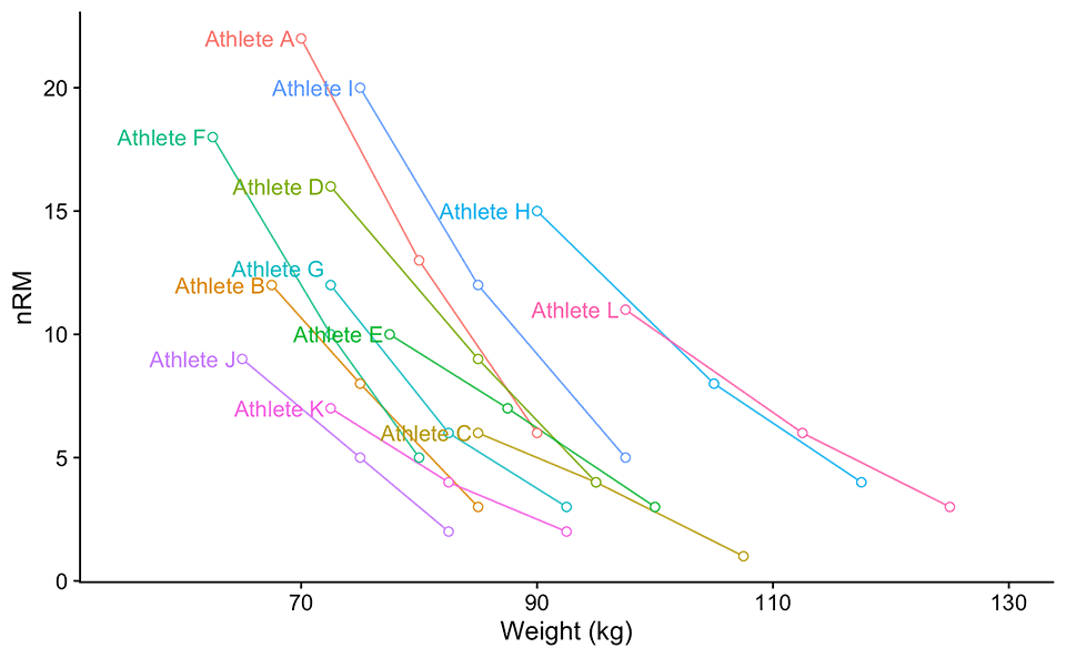
Figure 1: Reps to failure tests of the 12 athletes
All the model definitions explained in the previous part of this article series utilize %1RM as a predictor variable, but as alluded a few times so far, we do not know %1RMs because we do not know athletes’ 1RMs. This puzzled me for a brief period of time. If we do not know 1RMs, maybe we can estimate them? What I have done, is I have introduced another model parameter: 1RM (ideally we should call it est1RM to differentiate it from the observed 1RM). This additional parameter is being estimated together with k, kmod, or klin parameter. Table 2 contains model definitions using %1RM (or the models we have used so far), as well as model definitions that uses absolute weight instead.
Please note that Epley’s model estimates 0RM, not 1RM. I have tried different model definition, where 1RM is estimated: nRM = (k * 1RM + 1RM - w) / (k * w). Unfortunately, I had issues with parameter estimation. Maybe in the future, I will improve it, but in the meantime use Equation 1 to estimate 1RM from 0RM using Epley’s model.
\[\begin{equation}
1RM = \frac{0RM}{k + 1}
\end{equation}\]
Equations 1
| Model Name | Uses %1RM (one parameter estimated) | Uses Weight (two parameters estimated) |
|---|---|---|
| Epley | nRM = (1 – %1RM) / (k * %1RM) | nRM = (0RM – w) / (k * w), |
| Modified Epely | nRM = ((kmod – 1) * %1RM + 1) / (kmod * %1RM) | nRM = ((kmod – 1) * w + 1RM) / (kmod * w), |
| Linear/Brzycki’s | nRM = (1 – %1RM) * klin + 1 | nRM = (1 – (w / 1RM)) * klin + 1 |
Table 2: Model definitions. Original models utilize %1RM and estimate one parameter (either k, kmod, and klin). Model definitions utilizing absolute weight, on top of estimating k, kmod, or klin parameter, estimate additional one (i.e., 1RM)
To demonstrate how these models work, let’s take our Athlete C as an example. Table 3 shows estimated parameters for Epley’s, Modified Epley’s and Linear/Brzycki’s models, including estimated 1RMs and model performance metrics. Figure 2 depicts model predictions. Note that Epley’s and Modified Epley’s models have the same weight predictions, but note that they have different %1RM predictions (particularly for the observed 1RM; this is again due to weird mathematical characteristics of the original Epley’s model where 100% 1RM is at 0RM).
| Model | param | 1RM (kg) | MAE (Reps) | RMSE (Reps) | maxErr (Reps) | R2 |
|---|---|---|---|---|---|---|
| Epley | 0.0565 | 108.5 | 0.2287 | 0.2426 | -0.3431 | 0.9861 |
| Modified Epley | 0.0535 | 108.5 | 0.2287 | 0.2426 | -0.3431 | 0.9861 |
| Linear | 24.0328 | 107.8 | 0.0984 | 0.1045 | -0.1475 | 0.9974 |
Table 3: Estimated model parameters and model performance for the Athlete C. MAE = mean-absolute error; RMSE = root-mean-squared-error; maxErr = maximal error; IQR = error interquartile range; R2 = variance explained
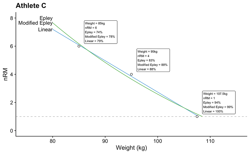
Figure 2: Model predictions for the Athlete C. Note that Epley’s and Modified Epley’s model have the same weights predictions, but note that they have different %1RM predictions (particularly for the observed 1RM; this is again due to weird mathematical characteristic of the original Epley’s model where 100% 1RM is at 0RM). Text in the boxes represent estimated %1RM using estimated k, kmod, or klin parameter
Compared to models using %1RM, which normalizes the individuals on the x-axis scale, using weight models for creating generic estimates is more tricky. We have few options. The simplest option is to make individual profiles and then average the k, kmod, or klin parameter to get the generic/pooled estimate. Better option is to use mixed-effects (or hierarchical) models (in this case non-linear mixed-effect models). Here we have two options. We can make estimated 1RM parameter to vary across individuals (i.e. to be random parameter). This is often called random-intercept model and in our case it is a wise choice (as can be seen from Figure 1). With this model, estimated k, kmod, or klin parameter will be fixed (i.e., same for everyone). Second option is to make both k, kmod, or klin and 1RM parameters random (this is called random-intercept and random-slope model). I will show you how to fit these models using the {STM} package 10 later in this article series.
How Can This Be Used in Practice
The practical implications of these models are instantly evident. If you have …
The practical implications of these models are instantly evident. If you have occasional plus set (a set taken to the point of technical failure, beyond the prescribed number of reps) 8, particularly if they are done with varying load and thus resulting number of repetitions, these can be plugged in aforementioned models to get not only estimated 1RM but also the individualized profile that can be used to prescribe training in the next phase. Of course, there are tricky assumptions depending on the time window during which these plus sets are collected: (1) assumption of the fixed 1RM, (2) assumption of the same technique, (3) assumption that the sets are really taken to failure under same emotional arousal, (4) assumption that there are no fatigue nor facilitation effects, nor interactions with other exercises, (5) assumption that there is no day-to-day variability in performance, (6) assumption that there is no measurement error, and (7) assumption that I have covered all assumptions (pun intended). These are all bold assumptions. But again, we are using these models as tools, not the truth. Later in this part of the article series, I will walk you through one collected training log to demonstrate how can these be applied.
What needs to be done, for this and for other applications that follow, is a validity study where we can compare 1RM predictions by the models to observed 1RM and check whether these are within practically significant difference. I might need to start working on papers since I have some data that can be used for this purpose (as soon as I finish writing some papers for my sprint profiling Ph.D. – it has been on the back burner for a while).
Knowing 1RM, but not taking sets to failure
Another scenario that might happen is knowing 1RM, but not taking sets to the point of failure. In this case, we do need to have some subjective rating that we can use. There are other options, like measuring concentric velocity (assuming maximal intent on each repetition), but that is the topic for another article. One such rating is perceived reps-in-reserve (pRIR) or subjectively estimated reps-in-reserved (eRIR). pRIR or eRIR is a simple number that lifter provides once the set is done and represents his or her estimate how many more reps are left in the tank. This estimate is of course imprecise 1 3 4 5 6 7 13 14 15 16 19 20 particularly for the large numbers (i.e., large eRIRs) and/or light loads, but it can still be useful.
Table 4 demonstrates one example of how eRIR can be used to estimate nRM or RTF (eRTF). For example, if I have done 5 reps, and I feel that I could have done 2 more (i.e., 2 eRIR), the estimated nRM is equal to 5 + 2, or 7RM. There are other options, like using rate-of-perceived-exertion (RPE), or even perceived percent of max reps (p%MR), which I think is very hard to estimate and quantify by perception, but in my humble opinion, nothing beats simplicity and athlete understandability of the eRIR scale.
| 1RM (kg) | Weight (kg) | %1RM | Reps | eRIR | eRTF |
|---|---|---|---|---|---|
| 95 | 85.0 | 0.8947 | 1 | 2 | 3 |
| 95 | 75.0 | 0.7895 | 7 | 1 | 8 |
| 95 | 67.5 | 0.7105 | 9 | 3 | 12 |
Table 4: Using perceived reps-in-reserve (eRIR) to supplement submax set with the aim to estimate reps-to-failure (eRTF, or estimated nRM)
The eRTF from Table 4 can be used instead of observed reps-to-failure and plugged in the models. In addition to this, if we know the measurement error of the eRIR scale for a particular movement, we can use SIMEX procedure 9 12 17 to estimate the profiles when there would be no measurement error. It bears repeating that these are tools not truth.
Using weighting
Not all sets are created equal – and this is particularly the case when we are using sub max sets with eRIR to estimate profiles. We will trust sets with low reps and low eRIR more than the sets with the high number of reps and/or high eRIR rating. We can use this knowledge when estimating profiles by weighting the observations. Weighting simply multiplies the residual of the observation (i.e., the difference between the observed and fitted/predicted value) with weight. In normal regression, each observation have a same weight. By using bigger weights for certain observations, we can give it more importance, which will pull the predictions more towards that data point.
Table 5 contains various weighting options we can use for profile estimation. Please note that reps are weighted as 1/reps, or in other words giving more weight to small number of repetition, while eRIR is weighted using 1/(eRIR + 1) to avoid division by zero. Table 6 contains relative (or normalized) weights, using the weight / min(weight). This approach show how many times certain observations are stronger than the lowest weighted observation.
Both {STM} package 10 and strengthPRO app allow you to perform all types of weighting. I am going to walk you through these option later in the article series.
| 1RM (kg) | Weight (kg) | %1RM | Reps | eRIR | eRTF | weighting: none | weighting: reps | weighting: load | weighting: eRIR | weighting: reps x load | weighting: reps x eRIR | weighting: load x eRIR | weighting: reps x load x eRIR |
|---|---|---|---|---|---|---|---|---|---|---|---|---|---|
| 95 | 85.0 | 89.5 | 1 | 2 | 3 | 1 | 1.0000 | 85.0 | 0.3333 | 85.00 | 0.3333 | 28.33 | 28.333 |
| 95 | 75.0 | 78.9 | 7 | 1 | 8 | 1 | 0.1429 | 75.0 | 0.5000 | 10.71 | 0.0714 | 37.50 | 5.357 |
| 95 | 67.5 | 71.1 | 9 | 3 | 12 | 1 | 0.1111 | 67.5 | 0.2500 | 7.50 | 0.0278 | 16.88 | 1.875 |
Table 5: Using non-linear regression to estimate our profiles and parameters, we can use different weighting strategies (i.e., giving more weight to different observations). This table provides absolute weights, while Table 6 contains relative weights
| 1RM (kg) | Weight (kg) | %1RM | Reps | eRIR | eRTF | weighting: none | weighting: reps | weighting: load | weighting: eRIR | weighting: reps x load | weighting: reps x eRIR | weighting: load x eRIR | weighting: reps x load x eRIR |
|---|---|---|---|---|---|---|---|---|---|---|---|---|---|
| 95 | 85.0 | 89.5 | 1 | 2 | 3 | 1 | 9.000 | 1.259 | 1.333 | 11.333 | 12.000 | 1.679 | 15.111 |
| 95 | 75.0 | 78.9 | 7 | 1 | 8 | 1 | 1.286 | 1.111 | 2.000 | 1.429 | 2.571 | 2.222 | 2.857 |
| 95 | 67.5 | 71.1 | 9 | 3 | 12 | 1 | 1.000 | 1.000 | 1.000 | 1.000 | 1.000 | 1.000 | 1.000 |
Table 6: Using non-linear regression to estimate our profiles and parameters, we can use different weighting strategies (i.e., giving more weight to different observations). This table provides relative weights, while Table 5 contains absolute weights
Not knowing 1RM, and not taking sets to failure
Analysis where 1RM is not known and sets are not taken to failure is pretty much analysis of training logs, particularly of the training logs that have eRIR rating for the sets not taken to failure. Table 7 contains one such session, where the individual did 8/6/4/2 single-wave workout 8. Using the 1RM models, together with estimating RTF or nRM using simple nRM = Reps + eRIR equation, can give us both an estimate of 1RM, as well as the rep-max profile.
| Weight (kg) | Reps | eRIR |
|---|---|---|
| 107.5 | 8 | 4 |
| 117.5 | 6 | 2 |
| 125.0 | 4 | 2 |
| 137.5 | 2 | 1 |
Table 7: Example 8/6/4/2 single-wave workout with eRIR ratings
Figure 4.1 depicts model predictions for the data from Table 7. Please note that if we only use reps done as a target variable (i.e., assuming they are RTF or nRM; these are triangles on the figure), we will get wrong estimates and predictions (dashed lines). For that reason, we add eRIR to the reps done to get estimated RTFs or estimated nRMs.
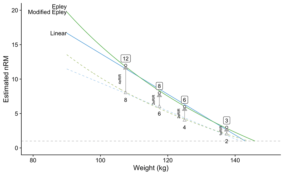
Figure 3: Model predictions for the data from Table 7. Note that triangles represent only reps are done, which are submaximal, and thus the profile estimations are off (dashed lines). Adding eRIR to reps done gives us estimated nRMs or estimated RTFs, which we can use to feed the models. There is no weighting used in these models. Please refer to Table 8 and Figure 4 for a summary of the weighted model estimates
Table 8 contains estimated 1RMs as well as profile parameters/coefficients using the Epley’s, Modified Epley’s, and Linear model with various types of observations weighting covered previously. For simple visual comprehension, this data can be depicted as box plots (Figure 5).
| model | weighting | coef | 1RM |
|---|---|---|---|
| Epley | eRIR | 0.0350 | 146.4 |
| Epley | load | 0.0344 | 146.0 |
| Epley | load x eRIR | 0.0352 | 146.5 |
| Epley | none | 0.0342 | 145.9 |
| Epley | reps | 0.0351 | 146.5 |
| Epley | reps x eRIR | 0.0357 | 146.8 |
| Epley | reps x load | 0.0352 | 146.6 |
| Epley | reps x load x eRIR | 0.0359 | 146.9 |
| Modified Epley | eRIR | 0.0338 | 146.4 |
| Modified Epley | load | 0.0333 | 146.0 |
| Modified Epley | load x eRIR | 0.0340 | 146.5 |
| Modified Epley | none | 0.0331 | 145.9 |
| Modified Epley | reps | 0.0339 | 146.5 |
| Modified Epley | reps x eRIR | 0.0345 | 146.8 |
| Modified Epley | reps x load | 0.0340 | 146.6 |
| Modified Epley | reps x load x eRIR | 0.0346 | 146.9 |
| Linear | eRIR | 40.7589 | 143.8 |
| Linear | load | 41.9201 | 143.2 |
| Linear | load x eRIR | 40.4123 | 143.9 |
| Linear | none | 42.2964 | 143.0 |
| Linear | reps | 40.5262 | 144.1 |
| Linear | reps x eRIR | 39.2496 | 144.6 |
| Linear | reps x load | 40.2074 | 144.2 |
| Linear | reps x load x eRIR | 38.9739 | 144.7 |
Table 8: 1RM and profile estimations using Epley’s, Modified Epley’s, and Linear model with various types of observations weighting
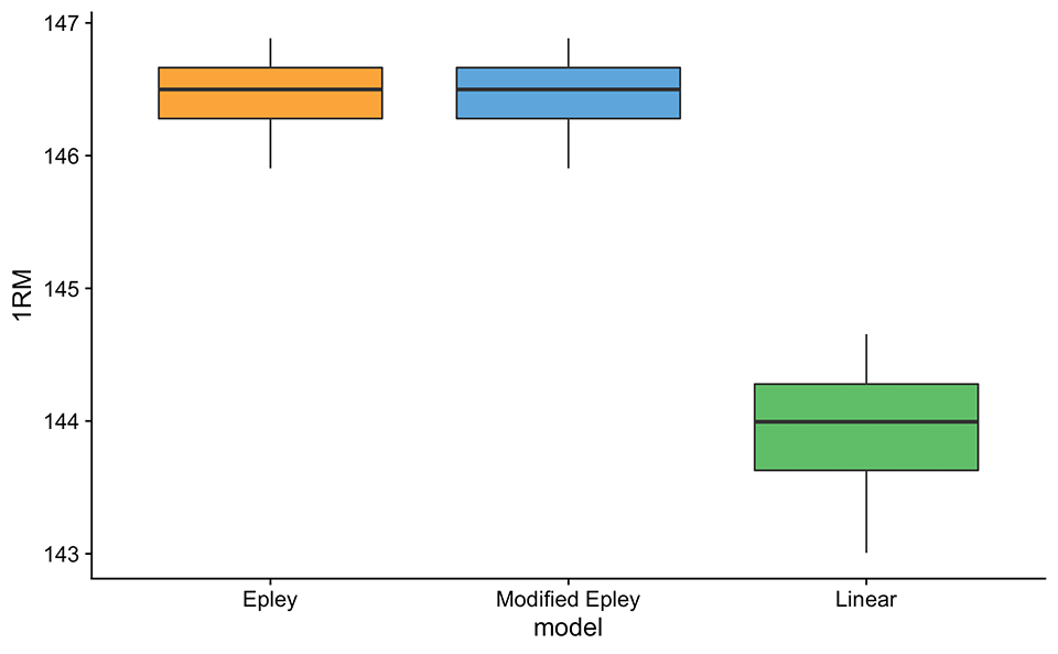
Figure 4: Box-plot of estimated 1RM using Epley’s, Modified Epley’s, and Linear model with various types of observations weighting. This is graphical summary of Table 8
I am not sure using single session log-data is a wise choice (unless it is designated testing session, which we want to avoid here) – it is better to use some type of rolling log analysis (RLA), where multiple sets are taken into analysis and we can get estimated changes or trends as well, for both parameter values, as well as 1RM. Table 10 contains sample of one such data collected over 12 weeks (please note that this data is fabricated, i.e., simulated by me for the purpose of example). This training program involves doing, say bench press, for two sessions a week, “Session A” and “Session B” (Table 9). Both session are double-wave scheme 8. Session A is more “extensive” and involves linear progression 8 across three weeks (Table 9), while Session B is more “intensive” and involve plateau progression 8, in which the reps stays the same, but the weight increase.
| Session | Week 1 | Week 2 | Week 3 |
|---|---|---|---|
| Session A | 2 x 12/10/8 | 2 x 10/8/6 | 2 x 8/6/4 |
| Session B | 2 x 5/3/1 | 2 x 5/3/1 | 2 x 5/3/1 |
Table 9: Training session involved in the training log (Table 10)
The training program consists of 4 phases, each 3 weeks long. Table 10 contains only a sample of the first phase. In addition to logging weight and reps done, individuals also logged eRIRs. eRIRs over 5 reps-in-reserve are not logged and are treated as NA (i.e., missing-value).
| phase | week | session | set | weight | reps | eRIR |
|---|---|---|---|---|---|---|
| 1 | 1 | Session A | 1 | 57.5 | 12 | |
| 2 | 62.5 | 10 | 5 | |||
| 3 | 70.0 | 8 | 3 | |||
| 4 | 55.0 | 12 | ||||
| 5 | 60.0 | 10 | ||||
| 6 | 65.0 | 8 | 4 | |||
| Session B | 1 | 72.5 | 3 | 4 | ||
| 2 | 80.0 | 2 | 3 | |||
| 3 | 87.5 | 1 | 2 | |||
| 4 | 77.5 | 3 | 3 | |||
| 5 | 85.0 | 2 | 2 | |||
| 6 | 92.5 | 1 | 1 | |||
| 2 | Session A | 1 | 62.5 | 10 | ||
| 2 | 67.5 | 8 | 4 | |||
| 3 | 77.5 | 6 | 3 | |||
| 4 | 60.0 | 10 | ||||
| 5 | 65.0 | 8 | 5 | |||
| 6 | 72.5 | 6 | 4 | |||
| Session B | 1 | 75.0 | 3 | 4 | ||
| 2 | 82.5 | 2 | 3 | |||
| 3 | 90.0 | 1 | 1 | |||
| 4 | 80.0 | 3 | 3 | |||
| 5 | 87.5 | 2 | 2 | |||
| 6 | 95.0 | 1 | 0 | |||
| 3 | Session A | 1 | 67.5 | 8 | 4 | |
| 2 | 75.0 | 6 | 3 | |||
| 3 | 85.0 | 4 | 1 | |||
| 4 | 65.0 | 8 | 5 | |||
| 5 | 72.5 | 6 | 4 | |||
| 6 | 80.0 | 4 | 2 | |||
| Session B | 1 | 77.5 | 3 | 4 | ||
| 2 | 85.0 | 2 | 3 | |||
| 3 | 92.5 | 1 | 1 | |||
| 4 | 82.5 | 3 | 3 | |||
| 5 | 90.0 | 2 | 2 | |||
| 6 | 97.5 | 1 | 0 |
Table 10: Training log of 4 phases, each 3 weeks long. Each week consists of two workouts: Session A, and Session B (Table 9). In addition to logging weight and reps done, individual also logged eRIRs. eRIRs over 5 reps-in-reserve are not logged and are treated as NA (i.e., missing-value). This table is only a sample, involving phase 1 of this training program log
Figure 5 depicts an analysis of the training log data using Epley’s, Modified Epley’s, and Linear’s models. But as you can see, this analysis provides an under-representation of the 1RM, as well as the profile. Why is so? Well, because we are using all sets, rather than the “best” sets. For example, let’s assume that the maximum in a given phase without fatigue and interactions from other previous exercises and previous sets is 80 x 8 @0eRIR. This also implies that if I lift that sub-maximally, e.g., 80 x 6 @2eRIR, this will also be my “best” performance (although not “manifested”). But let’s say that I feel tired from previous workouts, or I had a bad night’s sleep and I did 80 x 5 @1eRIR. This is indeed a drop in my “state.” Since these enter the model, we are not going to estimate the “best” profile, but some type of the “average” profile.
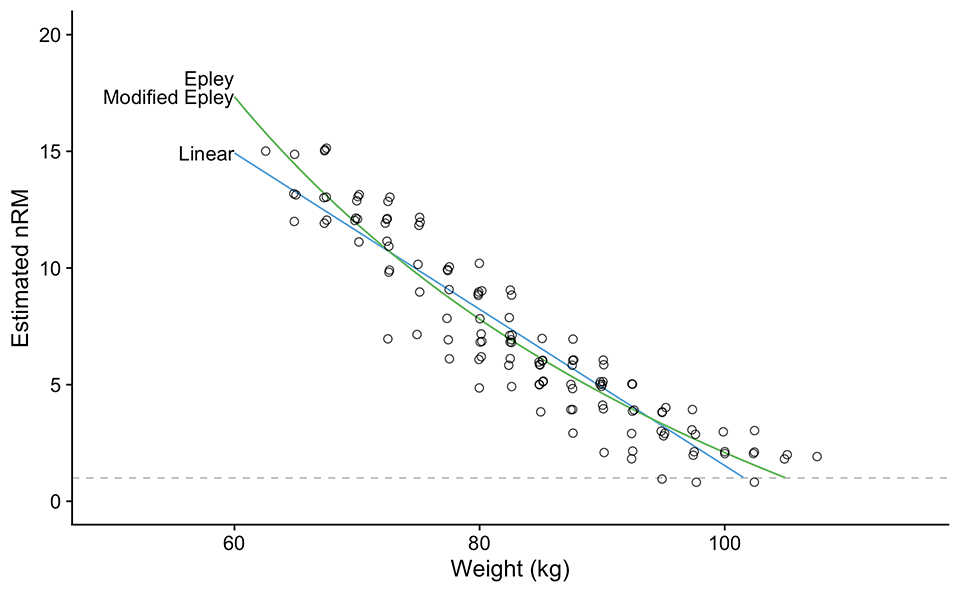
Figure 5: Analysis of the pooled training log data (Table 10). Unfortunately, this type of analysis (without any filter of what goes inside the model) under-estimates the profiles. Please note that I have added small jitter to the data points to show overlap where there are multiple sets of the same reps at the same weight across those 12 weeks
How do we solve this conundrum? Weighting the observations doesn’t help in this regard and might even make things worse. We can filter out top 5% of our best sets using weight x reps x (eRIR + 1) equation for multiple weight brackets. Figure 6 depicts one such analysis where we have filtered out the top 5% sets (using the aforementioned equation) across 10 weight brackets (i.e., we have split the weights used into 10 brackets). With this approach, we have filtered out the best sets across the weight range, and thus get some estimate of the “best” performance profile (across those 12 weeks).
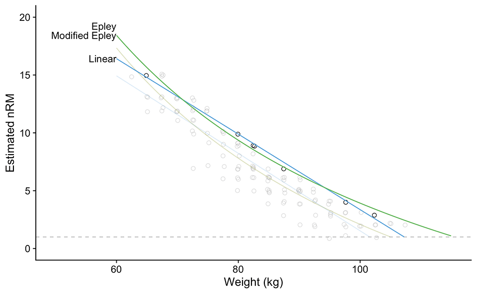
Figure 6: Re-analysis of training log data (Table 10 and Figure 5) by using top 5% sets across 10 weight brackets. Sets are rated using weight x reps x (eRIR + 1) equation
More elegant approach to solve this problem of filtering the best performance sets across weight continuum, is to use quantile non-linear regression 10 11. This approach is depicted on Figure 7 and it looks very similar to Figure 6.
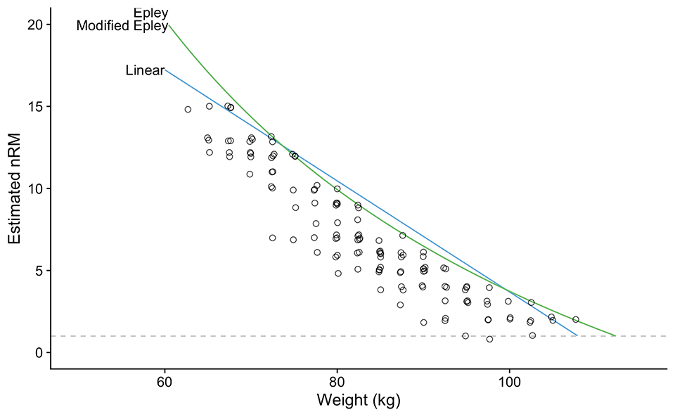
Figure 7: Re-analysis of training log data (Table 10 and Figure 5) by using quantile regression 10 11 with 0.95 percentile
Besides the analysis of the “best” performance (Figure 7 using 0.95 quantiles), we can also analyze the “worst” performance using 0.05 quantile (Figure 8). I came to this idea while writing this article, which is quite common to me, since writing is not a simple brain dump, but more importantly an exploration process. I am currently wrestling with this idea of minimum and maximum profile and what it implies. In my opinion, these are very related to the concept of pull the floor vs. push the ceiling 8. “Floor” in this example represents your worst performance, and collectively your worst profile. In other words, this is something that you might do on any day, but it can also be related to the shittiest performance due to fatigue, other sessions interactions, motivation, or variation. “Ceiling” on other hand is your best performance under the training program context. Since I have just “discovered” these, I am not sure yet what to think about it, but I do think it captures the “best” and the “worst” performance in a given program and context, which can be highly related to the pull the floor vs. push the ceiling concept.
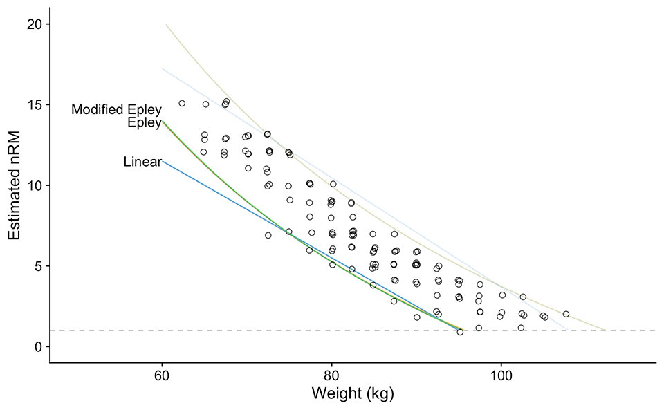
Figure 8: Re-analysis of training log data (Table 10 and Figure 5) by using quantile regression 10 11 with 0.05 percentile
So far we have analyzed our 12 weeks data as pooled, or everything together. Instead of simple “best” and “worst” profiles and estimated 1RMs across 12 weeks, we are also interested in trends over time, both in 1RM (is our athlete improving?) as well as profile (is our athlete able to do more reps at certain %1RM?). We also want to use these estimates to help us plan the next training phase. I am speculating, but in addition to this, the “best” vs “worst” performance profile trends can tell us some information about “pushing” vs. “pulling” or the “variability” or “range” in athlete performance (is the difference between best vs worst constant across time or does it changes? What does this mean? Are we managing workout stressors over time?). Again, remember that these analyses represent tools, not truth. But at least we have some “objectivish” data to use to complement our reasoning.
To achieve this, we can use rolling analysis. This might involve creating a rolling window of 3-4 weeks and then estimating 1RM and profile. Another option is to estimate these in time buckets, like phase to phase analysis. This is exactly what I have done in Figure 9, where the 0.95 and 0.05 quantile non-linear regression is applied across training phases. This analysis gives us “embedded” testing and some hints of the training effects (i.e., adaptation if the time windows are longer, or performance fluctuation if performance windows are shorter).
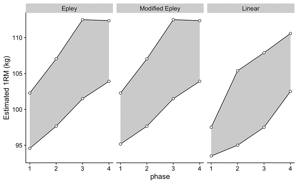
Figure 9: Estimated 1RMs across training phases using 0.95 and 0.05 percentile quantile non-linear regression
In addition to Figure 9, we can also plot the difference between the best and worst estimated 1RM across training phases (Figure 10). I am again speculating, but together with the trend of the worst performance from Figure 9, the difference can tell us whether we are managing the training well. My speculations can be found in Table 11 – please note that a very important piece of information that guides our interpretations is the time frame over which the analysis is taking place. This is something I am currently wrestling with, so if you have any hint of how this might be used, please do not hesitate to leave a comment below and contact me via other means. Not sure this analysis has been done yet, so I am not sure what to make out of it. We are in the process of exploration.
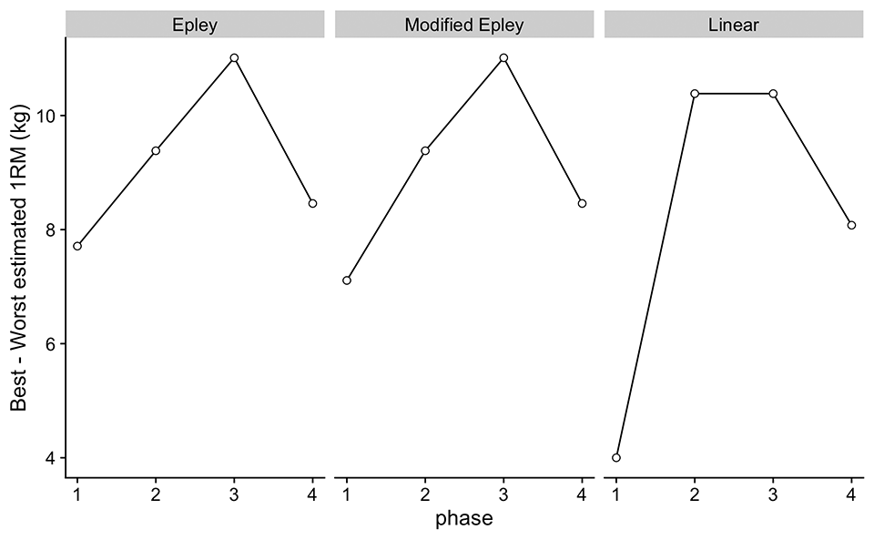
Figure 10: Plot of the best minus worst estimated 1RM from Figure 9
| Worst | Best | Difference | Meaning? |
|---|---|---|---|
| Constant | Constant | Constant | No change in adaptation nor performance? |
| Constant | Increasing | Increasing | Good peaking approach? No ‘pulling the floor’ (i.e. adaptation), but managing to manifest the best performance |
| Constant | Decreasing | Decreasing | No adaptation, but bad managing of the peaking day. Athlete unable to manifest the best performance due to bad managing of training stress? |
| Increasing | Constant | Increasing | Hmmm… weird? |
| Increasing | Increasing | Constant | This is PERFECT!! |
| Increasing | Decreasing | Increasing | Also weird… |
| Decresing | Constant | Increasing | Some negative effects, but athlete manages to manifest peaks |
| Decreasing | Increasing | Increasing | Could be effect of high training load causing bad days to be very bad, but athletes is able to manifest good performance within the analysis window? |
| Decreasing | Decreasing | Constant | Detraining |
Table 11: HIGHLY SPECULATIVE interpretations of the “best” vs “worst” estimated 1RMs
Embedded testing and Review and Retrospective
The Agile Periodization 8 approaches training from explore~exploit complementary aspects that are continuously integrated via short iterations and embedded testing using defined performance reviews and program retrospectives. The tools presented in this part of this article series can help us in analyzing the training program without designated testing days, although these testing days can be used occasionally to check the validity of this type of embedded testing. The great thing about these tools is that they can be used with both strength-specialists and strength-generalists. After a few weeks of “generic” progression tables, we can update our priors (Bayesian updating anyone? pun intended) using the provided tools and provide more individualized training prescriptions (given our assumptions). There are of course assumptions and errors involved, but this approach is a step in the right direction and not necessarily “exact truth” due to the “garbage-in garbage-out” phenomena.
Please correct me if I am wrong, but the tools outlined in this part are really novel and I plan to do a validity study from the data that we already have. If you intend to use these tools or ideas provided in this article, please reference them. You can reference this article part, as well as the {STM} package 10.
In the upcoming parts of this article series, I will walk you through the {STM} package 10 and show you how you can do this analysis yourself.
References
- Carzoli, Joseph P., Alex Klemp, Brittany Allman, Michael C. Zourdos, Jeong-Su Kim, Lynn B. Panton, and Michael J. Ormsbee. 2017. “Efficacy Of The Repetitions In Reserve-based Rating Of Perceived Exertion For The Bench Press In Experienced And Novice Benchers: 3644 Board #91 June 3 8.” Medicine & Science in Sports & Exercise 49 (May): 1041. https://doi.org/10.1249/01.mss.0000519859.98511.10
- Christian, Brian, and Tom Griffiths. 2017. Algorithms to Live by: The Computer Science of Human Decisions.
- Hackett, Daniel A., Stephen P. Cobley, Timothy B. Davies, Scott W. Michael, and Mark Halaki. 2017. “Accuracy in Estimating Repetitions to Failure During Resistance Exercise:” Journal of Strength and Conditioning Research 31 (8): 2162–68. https://doi.org/10.1519/JSC.0000000000001683.
- Hackett, Daniel A., Stephen P. Cobley, and Mark Halaki. 2018. “Estimation of Repetitions to Failure for Monitoring Resistance Exercise Intensity: Building a Case for Application.” Journal of Strength and Conditioning Research 32 (5): 1352–59. https://doi.org/10.1519/JSC.0000000000002419.
- Halperin, Israel, Tomer Malleron, Itai Har-Nir, Patroklos Androulakis-Korakakis, Milo Wolf, James Fisher, and James Steele. 2021. “Accuracy in Predicting Repetitions to Task Failure in Resistance Exercise: A Scoping Review and Exploratory Meta-Analysis.” Preprint. SportRxiv. https://doi.org/10.31236/osf.io/x256f.
- Helms, Eric R., John Cronin, Adam Storey, and Michael C. Zourdos. 2016. “Application of the Repetitions in Reserve-Based Rating of Perceived Exertion Scale for Resistance Training:” Strength and Conditioning Journal 38 (4): 42–49. https://doi.org/10.1519/SSC.0000000000000218.
- Hughes, Liam, Jeremiah Peiffer, and Brendan Scott. 2020. “Estimating Repetitions in Reserve in Four Commonly Used Resistance Exercises.” The Journal of Strength and Conditioning Research, September.
- Jovanović, Mladen. 2020a. Strength Training Manual: The Agile Periodization Approach. Independently published.
- Jovanović, Mladen. 2020b. Bmbstats: Bootstrap Magnitude-based Statistics for Sports Scientists
- Jovanović, Mladen. 2022. STM: Strength Training Manual r-Language Functions. Belgrade, Serbia. https://zenodo.org/record/6039086#.YhYdoejMKUk
- Koenker, Roger. 2022. Quantreg: Quantile Regression. https://CRAN.R-project.org/package=quantreg.
- Lederer, Wolfgang, and Helmut Küchenhoff. 2006. “A Short Introduction to the SIMEX and MCSIMEX.” R News 6 (January).
- Mansfield, Sean K., Jeremiah J. Peiffer, Liam J. Hughes, and Brendan R. Scott. 2020. “Estimating Repetitions in Reserve for Resistance Exercise: An Analysis of Factors Which Impact on Prediction Accuracy.” Journal of Strength and Conditioning Research Publish Ahead of Print (August). https://doi.org/10.1519/JSC.0000000000003779.
- Ormsbee, Michael J., Joseph P. Carzoli, Alex Klemp, Brittany R. Allman, Michael C. Zourdos, Jeong-Su Kim, and Lynn B. Panton. 2019. “Efficacy of the Repetitions in Reserve-Based Rating of Perceived Exertion for the Bench Press in Experienced and Novice Benchers:” Journal of Strength and Conditioning Research 33 (2): 337–45. https://doi.org/10.1519/JSC.0000000000001901.
- Perlmutter, Jared H., Jacob A. Goldsmith, Daniel M. Cooke, Ryan K. Byrnes, Michael H. Haischer, Jose C. Velazquez, Adam Sayih, Eric R. Helms, Chad Dolan, and Michael C. Zourdos. 2017. “Total Repetitions Per Set Effects Repetitions in Reserve-based Rating of Perceived Exertion Accuracy: 3648 Board #95 June 3 8.” Medicine & Science in Sports & Exercise 49 (May): 1043. https://doi.org/10.1249/01.mss.0000519863.21383.4c.
- Steele, James, Andreas Endres, James Fisher, Paulo Gentil, and Jürgen Giessing. 2017. “Ability to Predict Repetitions to Momentary Failure Is Not Perfectly Accurate, Though Improves with Resistance Training Experience.” PeerJ 5 (November): e4105. https://doi.org/10.7717/peerj.4105.
- Wallace, Michael. 2020. “Analysis in an Imperfect World.” Significance 17 (1): 14–19. https://doi.org/10.1111/j.1740-9713.2020.01353.x.
- White, John Myles. 2013. Bandit Algorithms for Website Optimization. Developing, Deploying, and Debugging. Sebastopol, California: O’Reilly.
- Zourdos, Michael C., Jacob A. Goldsmith, Eric R. Helms, Cameron Trepeck, Jessica L. Halle, Kristin M. Mendez, Daniel M. Cooke, et al. 2019. “Proximity to Failure and Total Repetitions Performed in a Set Influences Accuracy of Intraset Repetitions in Reserve-Based Rating of Perceived Exertion:” Journal of Strength and Conditioning Research, February, 1. https://doi.org/10.1519/JSC.0000000000002995.
- Zourdos, Michael C., Alex Klemp, Chad Dolan, Justin M. Quiles, Kyle A. Schau, Edward Jo, Eric Helms, et al. 2016. “Novel Resistance Training–Specific Rating of Perceived Exertion Scale Measuring Repetitions in Reserve:” Journal of Strength and Conditioning Research 30 (1): 267–75. https://doi.org/10.1519/JSC.0000000000001049.
Related Articles

Load-Exertion Tables And Their Use For Planning – Part 4
In the previous part, we used a set of Epley’s equations to estimate both group and individual reps-max profiles, as well as to create progression tables. One characteristic of Epley’s equation is that 100% 1RM is achieved with 0RM, which is not an ecologically valid assumption. What the hell is 0RM in the first place? Find out in the…
Reps at 80% 1RM? Can They Be Useful for Individualizing Reps-Max Table?
The more weight you put on the bar, the less reps you are able to do. This is common knowledge and a phenomenon we want to describe, predict and intervene upon. However, this relationship tends to differ between individuals and exercises.

Load-Exertion Tables And Their Use For Planning – Part 1
Prescribing strength training is indeed tricky. Things tend to vary across lifts/movements, individuals, gender, rep ranges, types of programs, splits, and so forth. But we are not completely clueless. Find out the potential solution in the following article.

Load-Exertion Tables And Their Use For Planning – Part 3
In this article, I will teach you how to create individualized progression tables, but before we jump straight into that, I will walk you through the process of getting Epley’s 0.0333 coefficient in the first place.


Responses