Load-Exertion Tables And Their Use For Planning – Part 3
Individual Differences
Before I changed my Ph.D. topic to sprint profiling, I wanted to wrestle with velocity-based training (VBT). Although I am still interested in VBT, due to practical reasons, I have changed my topic to something more doable and probably more impactful. But anyway, for my VBT Ph.D., we have collected some interesting data (these will be the topic of another article or even scientific paper, although one paper is already published; see Jovanovic and Jukic 2). Some of those data involved performing max reps at 90 and 80% 1RM using the hex bar deadlift exercise. We have witnessed athletes that could perform up to 20 reps at 80% 1RM and athletes who could do 5 reps. “Yeah Mladen, but maybe you have used the wrong 1RM to base those %1RM percentages off?” Not so – we have tested and witnessed 1RM attempts as well.
Long story short – there are huge individual differences in max reps – %1RM relationship (i.e., Reps-Max Table/Relationship). These vary across individuals, but also within individuals depending on the experience, strength level, exercise, and so forth. For example, you might do 10 reps with 80% 1RM in the squat, but only 5 in the bench press. Even if you observe single exercises across time, the number of reps at fixed %1RM might vary across time due to changes in strength level (i.e., 1RM) or training type being done. For example, when you lifted 100kg in the bench press, you could do 5 reps at 85%, now when you lift 140kg you can do 3 reps at 85%. This makes generic max reps equations rubbish, right?
Hold your horses – although they are imprecise, generic equations (like the one we have explored in this article series) are still useful. Imagine you have 30 athletes, and you implement 10 exercises. That is 300 exercise-athletes combinations! There is no chance we are going to create the specific rep-max table for each. Thus, we use heuristics, in this case, generic equations and tables, but we should also allow for some wiggle room when prescribing, taking into account individual variations across days, as well as the model error 5. We just need to keep in mind that these equations are not precise and we need to balance out the costs of over-and under-shooting 5.
There are cases when having individual rep-max tables and profiles is useful and practically doable. This is especially useful for strength specialists and for the limited number of exercises (e.g., bench press, deadlift, and squat for a powerlifter) mostly during the push the ceiling type of programs.
In this article, I will teach you how to create individualized progression tables (I am also developing a web tool called strengthPRO that allows you to do everything covered in this article series with few mouse clicks), but before we jump straight into that, I will walk you through the process of getting that Epley’s 0.0333 coefficient in the first place. Once you understand this, as well as other models we could utilize, it will be very easy to apply it to single individuals (it will be especially easy using the strengthPRO app).
How did we get that 0.0333?
How would we approach the problem of estimating the relationship between max reps and %1RM for a single exercise, let’s say a bench press? One way to do it, the most common one, would be to recruit multiple athletes willing to suffer for a few training sessions. The first thing that needs to be done is to estimate individuals’ 1RMs (later in the article, I will show you how you can avoid this by using a novel approach). We do need to make sure that these 1RMs are stable across testing sessions, and do not vary much due to motivation, fatigue, or adaptation. These are our theoretical assumptions of course, and things do suffer from measurement error, like it or not.
The second thing to do, once we know the individuals’ 1RMs, is to perform a few sets to failure, for example using 90, 80, and 70% 1RM. Should these be done on the same day? In that case, the fatigue from the previous set will affect the following sets’ performance. If we do them across multiple days, will 1RM be stable enough? Should we randomize the set order? These are all practical questions that impose different assumptions and introduce different measurement errors. But for the sake of this article, I will not delve much into these, but assume there is no measurement error or interference.
Table 1 contains one such data set. We have 12 athletes performing three sets to failure using 90, 80, and 70% 1RM. From Table 1 we can see that the range for 90% is 2-6 reps, 4-13 reps for 80%, and 6-21 reps for 70% 1RM load. This is of course simulated data, but not too far from what you can observe in the wild.
| Athlete | 1RM | 90% | 80% | 70% |
|---|---|---|---|---|
| Athlete A | 100.0 | 6 | 12 | 21 |
| Athlete B | 95.0 | 4 | 8 | 13 |
| Athlete C | 120.0 | 2 | 4 | 6 |
| Athlete D | 105.0 | 4 | 9 | 17 |
| Athlete E | 110.0 | 2 | 6 | 11 |
| Athlete F | 90.0 | 5 | 9 | 18 |
| Athlete G | 102.5 | 3 | 7 | 11 |
| Athlete H | 130.0 | 4 | 8 | 15 |
| Athlete I | 107.5 | 4 | 13 | 20 |
| Athlete J | 92.5 | 3 | 5 | 9 |
| Athlete K | 102.5 | 2 | 4 | 7 |
| Athlete L | 140.0 | 3 | 6 | 11 |
Table 1: Athletes with different 1RMs performing three sets to failure using 90, 80, and 70% 1RM. Numbers in the table represent count of the maximum number of reps
Figure 1 represents a visual depiction of Table 1. “But why do %1RM vary across athletes? Shouldn’t they be exactly the same?” you might ask. Here is how it works in the wild (i.e., real-life). Let’s say the athlete’s 1RM is 110 kg, and we plan to do a set of 80% 1RM to failure. To estimate weight than needs to be used, we multiply 110 kg with 80%, or 110 * 0.8 which is equal to 88kg. Unfortunately, we only have 1.25kg plates, so our weight can only be a multiple of 2.5kg (i.e., 1.25 on each side, which gives us 2.5kg increments). So we decided to go with 85 kg as a set to failure. Then we need to re-calculate the %1RM, which is equal to 85 / 110, or 77.2%. Please note that we have a similar issue with 1RM estimation, and this also contributes to the measurement error.
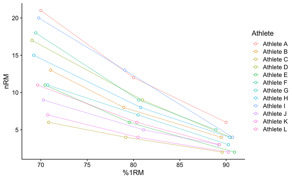
Figure 1: Visual representation of the Table 1. %1RMs used are not exactly the same for every athlete due to rounding of the weight (please check the main text for more info)
What we need to do next, is to decide what model we want to fit the data. Although we could fit a simple regression line, which has intercept and slope parameters/coefficients (we are going to introduce and use a modified linear model later in the next part of this article series), let’s go with Epley’s Equation 1 to showcase how k=0.0333 emerged.
\[\begin{equation}
nRM = \frac{1 – \%1RM}{k \times \%1RM}
\end{equation}\]
Equation 1
From the Equation 1, you can see that we need to estimate the k parameter, that minimizes the differences between predicted nRM and observed nRM. Since we have only one parameter to estimate (i.e., k), we would need only two sets to failure (i.e., 90 and 80% 1RM), although we have done three sets to failure in this example. On a side-note, if we use linear regression, we will need to estimate slope and intercept which would demand three sets to failure, and also have other issues, that I will cover in the next part of this article series, as well as provide an alternative.
Estimation of the k parameter in Equation (2.1) is the problem of non-linear regression or optimization. As alluded previously, we need to find the k value that minimizes the differences between observed nRMs and equation predicted nRMs (i.e., the residuals). These differences are often summarized or aggregated using the mean-squared-error (MSE), which is equal to \(MSE = \frac{\sum(nRM_{obs} – nRM_{pred})^2}{n}\), where \(nRM_{pred} = \frac{1 – \%1RM}{k \times \%1RM}\). We thus want to find the k that minimizes the MSE.
One way to do this, is to use the Optimization tool in the Microsoft Excel. This is cumbersome, especially if we need to repeat this for multiple athletes. Much more easier, more powerful, completely free, and reproducible way is to do this is in the R language 7 using the stats::nls function. I have developed a whole R package, STM, short of Strength Training Manual, to help me perform all these estimations and set and rep schemes building 4. This whole article series was written in the R Markdown 8 9 with the help of the STM package. Without going any deeper in the estimation and optimization, I recommend checking my bmbstats book 6 and R package 3 for more info about these and other topics.
One thing I need to address before we move away from these braniac topics: please note that the Equation 1 have nRM as target variable, and %1RM as predictor. Although we could reverse these variables (see Equation 2), using nRM as target variable (Equation 1) is a proper statistical procedure, since %1RM is independent or given value, while number of reps performed is dependent variable. Note that estimated k parameter from reversed model (Equation 2) will not be exactly the same as the k parameter estimated using nRM as target variable and %1RM as predictor.
\[\begin{equation}
\%1RM = \frac{1}{k \times nRM + 1}
\end{equation}\]
Equation 2
Flipping the dependent and independent variables is a common mistake (which I have done myself numerous times). Although we will use Equation 2 to estimate %1RM from target reps, the statistically correct model definition to estimate k parameter is using Equation 1, where nRM is a target variable.
Using the data from Table 1 and Figure 1, estimated k parameter value is 0.032. It is easier to understand this visually. Figure 2 depicts model predictions as a black line. What you need to notice is how more variable is the residuals with the lower %1RM. This is why the 1RM prediction equations, like Epley’s \(1RM = (Reps \times Weight \times 0.0333) + Weight\) lose precision the more reps are being done (i.e., the lower %1RM is being used).
Another thing to notice in Figure 1 is the characteristic of Epley’s model (Equation 1) where 0RM is achieved with 100 %1RM. This is the mathematical property of Equation 1 and there is nothing we can do about it using this equation format (we will fix it with modified Epley’s equation in the next part of this article series). I am not sure why they have chosen this equation where 0RM is at 100% 1RM (i.e., the line origin is at 0RM and 100%RM), instead of 1RM at 100% 1RM. If someone has some info, please let me know.
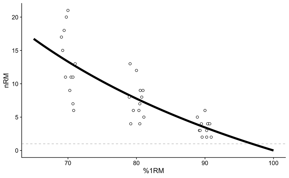
Figure 2: Generic or pooled model fit. This approach uses all the athletes to estimate the “average” profile
To quantify model performance, we need to analyze the residuals. I am going to use five estimators: (1) mean-absolute-error (MAE), (2) root-mean-squared-error (RMSE), (3) maximal error (maxErr), (4) error interquartile range (IQR), and (5) variance explained (\(R^2\)) 6. You can find these in Table 2.
| MAE (Reps) | RMSE (Reps) | maxErr (Reps) | IQR (Reps) | R2 |
|---|---|---|---|---|
| 2.38 | 3.11 | -7.68 | 3.16 | 0.636 |
Table 2: Generic/Pooled model performance on the training data set. MAE = mean-absolute error; RMSE = root-mean-squared-error; maxErr = maximal error; IQR = error interquartile range; R2 = variance explained
Please note that the model performance (Table 2) is evaluated on the training data set, i.e., the very same data that we have used to fit the model. Ideally, we want to evaluate the model performance on the hold-out or unseen data, often referred to as testing data set. This can be done by removing few athletes from the training data, then estimating how good the model predicts for them. This loop can be done multiple times using the cross-validation, or performing the prediction for every athlete using the leave-one-out cross-validation (LOOCV) 6. This testing data set performance is often worse than the training data set performance. Estimating model performance on unseen data is unfortunately still not used in sport science research is satisfactory degree. But let’s move on from this topic, since it is not really important for the discussion of creating individualized regression tables. Just keep in mind that we want to evaluate model performance on unseen data, since we are going to use this generic model on new athletes, or athletes unseen by the model, so we are interested in knowing how it performs on new athletes/data, not on athletes/data we have used to build the model in the first place.
What can we conclude about this model performance (Table 2)? In short – it is shit. MAE, or mean absolute difference is equal to 2.38 reps, where the biggest error is equal to -7.68 reps. Table 3 contains model performance estimators for each athlete separately, and they are even more shittier. As can be seen, the generic model can only be useful for the Athlete B only (please check model performance using his/here testing data).
| Athlete | MAE (Reps) | RMSE (Reps) | maxErr (Reps) | IQR (Reps) |
|---|---|---|---|---|
| Athlete A | 4.82 | 5.27 | -7.68 | 2.57 |
| Athlete B | 0.32 | 0.32 | -0.34 | 0.32 |
| Athlete C | 4.20 | 4.70 | 6.80 | 2.59 |
| Athlete D | 1.83 | 2.06 | -3.07 | 1.17 |
| Athlete E | 1.71 | 1.76 | 2.04 | 0.46 |
| Athlete F | 2.31 | 2.72 | -4.32 | 1.60 |
| Athlete G | 0.92 | 1.14 | 1.86 | 0.75 |
| Athlete H | 0.83 | 0.86 | -1.18 | 0.29 |
| Athlete I | 4.04 | 4.69 | -6.53 | 2.86 |
| Athlete J | 2.39 | 2.76 | 4.15 | 1.69 |
| Athlete K | 3.59 | 4.03 | 5.86 | 2.25 |
| Athlete L | 1.63 | 1.79 | 2.55 | 0.91 |
Table 3: Generic/Pooled model performance estimated for each individual athlete. MAE = mean-absolute error; RMSE = root-mean-squared-error; maxErr = maximal error; IQR = error interquartile range; R2 = variance explained
Although shit for predicting individual nRMs and 1RMs, generic equation such as this one are still useful (as alluded previously), since it gives us hints on the general pattern, which we can use in training prescription. Table 4 contains Rep-Max table using the estimated k parameter and Epley’s Equation 3 that we can use to gain some insights for prescription.
\[\begin{equation}
\%1RM = \frac{1}{0.032 \times nRM + 1}
\end{equation}\]
Equation 3
| Reps | 1 | 2 | 3 | 4 | 5 | 6 | 7 | 8 | 9 | 10 | 11 | 12 | 13 | 14 | 15 |
| %1RM | 96.9 | 94 | 91.2 | 88.6 | 86.1 | 83.8 | 81.6 | 79.5 | 77.5 | 75.7 | 73.9 | 72.1 | 70.5 | 68.9 | 67.5 |
Table 4: Generic/Pooled Rep-Max Table
This is, in short, the story of how we got that 0.0333 k parameter, although we didn’t get exactly the same number, you get the idea. Although far from great, these generic models are still useful as heuristics when dealing with unknown exercises, unknown athletes, a large number of both, when we do not need to be very precise, or when we supplement our numbers with coaching wisdom or individual feedback.
Instead of pooling everyone together to get the generic profile (or “average” profile), we can estimate individual profiles, or in this case k parameter values. Let’s do that in the next section of the article.
Individual Models
Figure 3 depicts individual profiles, estimated using Epley’s model definition (Equation 1). Figure 3 also depicts a generic (or pooled) profile as a grey line. As you can see, only Athlete B is very similar to the generic profile. Also, note that all profiles originate from 0RM and 100%. Individual estimated k parameter values are also depicted on Figure 3, including the model performance for every athlete.
.
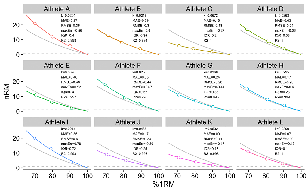
Figure 3: Individual profiles. Grey line indicated the previously estimated generic/pooled profile. MAE = mean-absolute error; RMSE = root-mean-squared-error; maxErr = maximal error; IQR = error interquartile range; R2 = variance explained
If you compare the performance values from Figure 3 to generic performance values (Tables 2 and 3), you can quickly note a much better fit (the simple visual check of Figure 3 will also tell you the same story). One thing to keep in mind is that even if we use the individual models, the fit will probably not be perfect (i.e., all points on the line). Additionally, this model that we have utilized (i.e., Epley’s Equation 1) might even be biased or systematically wrong for some individuals. In other words, they might not follow the relationship as assumed by this model.
In addition to these two modeling extremes, i.e., pooled vs. individual model, one might opt for a mixed model, which can be used for both tasks (i.e., generic/pooled profile and individual profiles), plus it works with missing data (e.g., few athletes missing few sets). Discussing these is beyond the scope of this article, and to be honest, beyond my knowledge (I can fit mixed models in R without any issues, but I am still learning all the nuts and bolts of how they work).
Table 6 contains individual rep-max tables, created from estimated individual k parameter values and Equation 2.
| Athlete | 1 | 2 | 3 | 4 | 5 | 6 | 7 | 8 | 9 | 10 | 11 | 12 | 13 | 14 | 15 |
|---|---|---|---|---|---|---|---|---|---|---|---|---|---|---|---|
| Athlete A | 98.0 | 96.1 | 94.2 | 92.5 | 90.7 | 89.1 | 87.5 | 86.0 | 84.5 | 83.0 | 81.7 | 80.3 | 79.0 | 77.8 | 76.6 |
| Athlete B | 96.9 | 94.0 | 91.3 | 88.7 | 86.3 | 84.0 | 81.8 | 79.7 | 77.8 | 75.9 | 74.1 | 72.4 | 70.8 | 69.2 | 67.7 |
| Athlete C | 93.7 | 88.2 | 83.2 | 78.8 | 74.9 | 71.3 | 68.0 | 65.0 | 62.3 | 59.8 | 57.5 | 55.4 | 53.4 | 51.5 | 49.8 |
| Athlete D | 97.4 | 95.0 | 92.7 | 90.5 | 88.4 | 86.4 | 84.4 | 82.6 | 80.8 | 79.2 | 77.5 | 76.0 | 74.5 | 73.1 | 71.7 |
| Athlete E | 96.2 | 92.7 | 89.4 | 86.3 | 83.5 | 80.8 | 78.3 | 75.9 | 73.7 | 71.6 | 69.6 | 67.8 | 66.0 | 64.3 | 62.7 |
| Athlete F | 97.6 | 95.2 | 93.0 | 90.9 | 88.9 | 87.0 | 85.1 | 83.4 | 81.7 | 80.0 | 78.5 | 77.0 | 75.5 | 74.1 | 72.8 |
| Athlete G | 96.5 | 93.1 | 90.1 | 87.2 | 84.5 | 81.9 | 79.5 | 77.3 | 75.1 | 73.1 | 71.2 | 69.4 | 67.7 | 66.0 | 64.5 |
| Athlete H | 97.1 | 94.4 | 91.9 | 89.4 | 87.1 | 85.0 | 82.9 | 80.9 | 79.0 | 77.2 | 75.5 | 73.8 | 72.3 | 70.8 | 69.3 |
| Athlete I | 97.9 | 95.9 | 94.0 | 92.1 | 90.3 | 88.6 | 87.0 | 85.4 | 83.8 | 82.3 | 80.9 | 79.5 | 78.2 | 76.9 | 75.7 |
| Athlete J | 95.6 | 91.5 | 87.8 | 84.3 | 81.1 | 78.2 | 75.4 | 72.9 | 70.5 | 68.3 | 66.2 | 64.2 | 62.3 | 60.6 | 58.9 |
| Athlete K | 94.4 | 89.4 | 84.9 | 80.9 | 77.2 | 73.8 | 70.7 | 67.9 | 65.2 | 62.8 | 60.6 | 58.5 | 56.5 | 54.7 | 53.0 |
| Athlete L | 96.2 | 92.6 | 89.3 | 86.2 | 83.4 | 80.7 | 78.2 | 75.8 | 73.6 | 71.5 | 69.5 | 67.6 | 65.8 | 64.2 | 62.6 |
Table 6: Individual Rep-Max Tables
As alluded to previously, these individualized Rep-Max tables can be useful for strength-specialists when utilizing a small number of exercises. Once we know these individuals’ k values, it is easy to plug them into the equations introduced in the previous parts to get individualized progression tables. Or use the strengthPro app.
The problem, however, is the time, effort, and energy it takes to create an individualized progression table. You need to select a few exercises, perform 1RM tests, then perform two or more sets to failure for every exercise. But there might be hope. I will introduce the novel method in the next part of this article.
Fast-Twitch Vs. Slow-Twitch and the Progression Increments
Having dissected many existing cycles and analyzed lifters’ training logs, their successes, and their failures, we have come to the conclusion that the “height” of the weekly weight jump must be adjusted to each lifter’s strength endurance. As a rule, the more “fast-twitch” you are, the bigger your jumps are.
There is this myth or urban legend regarding the number of reps done at 80% 1RM indicating whether someone is fast-twitch or slow-twitch individual. Although there is a recent study showing that “the number of completed repetitions at 80% of 1RM is moderately correlated with muscle fiber composition” 1, one quick glimpse at the graph they have provided will quickly let you know that this conclusion is rubbish (also one more example of researchers not using hold-out data sets). Besides this, I think it is detrimental to stamp someone with a fast-twitch or slow-twitch label based on the number of reps in a single exercise. Thinking logically, would this “label” hold across different exercises and movement patterns?
Even if complete bullshit, it might be worthwhile inspecting how the number of reps at 80% 1RM plays out with individualized progression tables. Not because this indicates fast- or slow-twitch individuals, but because it represents a snapshot of different individual profiles. In the Reload book 10, Fabio Zonin and Pavel Tsatsouline recommend adjusting weekly progressions based on the reps done at 80% 1RM (Table 7).
| nRM with 80% 1RM | %1RM Increment |
|---|---|
| ≥10 | 2% |
| 9-10 | 3% |
| 6-8 | 4% |
| ≤5 | 5% |
Table 7: Heuristic table provided by Fabio Zonin and Pavel Tsatsouline in the Reload book 10. Smaller the number of reps done at 80% 1RM, the bigger the progression step-to-step increments in %1RM, and vice versa
Reload book 10 by Fabio Zonin and Pavel Tsatsouline is one interesting read, and if you are interested in setting up 5×5 cycles please make sure to check it out. What I want to explore here, is whether progression steps vary for individuals doing high vs. a low number of reps at 80% (or in other words, individuals with different rep-max profiles), using progression tables outlined in the previous parts of this article. Let’s take our Athlete A, Athlete B, and Athlete C (Table 8) to explore this topic further.
| Athlete | 1RM | 90% | 80% | 70% |
|---|---|---|---|---|
| Athlete A | 100 | 6 | 12 | 21 |
| Athlete B | 95 | 4 | 8 | 13 |
| Athlete C | 120 | 2 | 4 | 6 |
Table 8: Three archetypal athletes we are going to use to explore how different number of reps at 80% 1RM plays out with different progression tables
These three athletes (Table 8) represent extreme archetypes: Athlete A has great, let’s call it strength-endurance, although I am not sure this means anything more than “able to do more reps at 80%.” Athlete B is our “Epley Guy,” which is very close to the generic profile, or simply our “average bloke.” Athlete C has really crappy strength endurance. Figure 4 depicts their individual profiles (these are the same as in Figure 3, but here I’ve selected only three of them to remove the clutter).
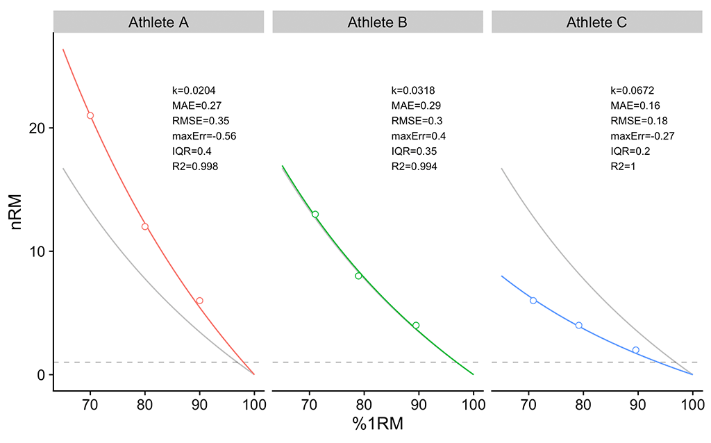
Figure 4: Individual profiles for Athlete A, B, and C. Grey line indicates “generic” or “pooled” profile estimated by using all 12 athletes
Once we have their individual profiles (i.e., estimated k parameter values using Epley’s model/equation), we can proceed and plug those into progression tables. Before we do that, let’s generate individual reps-max tables (Table 9).
| Athlete | 1 | 2 | 3 | 4 | 5 | 6 | 7 | 8 | 9 | 10 | 11 | 12 | 13 | 14 | 15 |
|---|---|---|---|---|---|---|---|---|---|---|---|---|---|---|---|
| Athlete A | 98.0 | 96.1 | 94.2 | 92.5 | 90.7 | 89.1 | 87.5 | 86.0 | 84.5 | 83.0 | 81.7 | 80.3 | 79.0 | 77.8 | 76.6 |
| Athlete B | 96.9 | 94.0 | 91.3 | 88.7 | 86.3 | 84.0 | 81.8 | 79.7 | 77.8 | 75.9 | 74.1 | 72.4 | 70.8 | 69.2 | 67.7 |
| Athlete C | 93.7 | 88.2 | 83.2 | 78.8 | 74.9 | 71.3 | 68.0 | 65.0 | 62.3 | 59.8 | 57.5 | 55.4 | 53.4 | 51.5 | 49.8 |
Table 9: Reps-Max table for the three archetypal athletes with different number of reps at 80%
The next step is to explore how these individual profiles play out using progression tables introduced in the previous part of this article. I will use sets of 3, 5, and 10 using the normal variant.
Table 10 contains different progressions for the sets of 3 using individual profiles. As can be seen, only Relative Intensity, RIR 2, RIR Increment, %MR Step Const, and %MR Step Var demonstrate variable progression increments for athletes with different profiles. The scenario is the same for the sets of 5 (Table 11) and sets of 10 (Table 12). Please note that the Relative Intensity approach in this example has actually the opposite increments to those recommended by Zonin and Tsatsouline. I will leave you to make your own conclusion.
| Scheme | Method | Athlete | Step 1 | Step 2 | Step 3 | Step 4 | Step 2-1 Diff | Step 3-2 Diff | Step 4-3 Diff |
|---|---|---|---|---|---|---|---|---|---|
| 3 x 3 (normal) | Deducted Intensity 2.5% | Athlete A | 84.2 | 86.7 | 89.2 | 91.7 | 2.50 | 2.50 | 2.500 |
| Athlete B | 81.3 | 83.8 | 86.3 | 88.8 | 2.50 | 2.50 | 2.500 | ||
| Athlete C | 73.2 | 75.7 | 78.2 | 80.7 | 2.50 | 2.50 | 2.500 | ||
| Relative Intensity | Athlete A | 73.0 | 77.7 | 82.5 | 87.2 | 4.71 | 4.71 | 4.712 | |
| Athlete B | 70.8 | 75.3 | 79.9 | 84.5 | 4.57 | 4.57 | 4.565 | ||
| Athlete C | 64.5 | 68.7 | 72.8 | 77.0 | 4.16 | 4.16 | 4.161 | ||
| Perc Drop | Athlete A | 82.4 | 85.4 | 88.3 | 91.3 | 2.96 | 2.96 | 2.955 | |
| Athlete B | 79.5 | 82.4 | 85.4 | 88.3 | 2.96 | 2.96 | 2.955 | ||
| Athlete C | 71.4 | 74.4 | 77.3 | 80.3 | 2.96 | 2.96 | 2.955 | ||
| RIR 2 | Athlete A | 81.7 | 84.5 | 87.5 | 90.7 | 2.82 | 3.02 | 3.241 | |
| Athlete B | 74.1 | 77.8 | 81.8 | 86.3 | 3.66 | 4.04 | 4.485 | ||
| Athlete C | 57.5 | 62.3 | 68.0 | 74.9 | 4.82 | 5.70 | 6.841 | ||
| RIR Increment | Athlete A | 86.1 | 87.9 | 89.8 | 91.8 | 1.83 | 1.91 | 1.990 | |
| Athlete B | 79.9 | 82.4 | 85.0 | 87.8 | 2.47 | 2.63 | 2.803 | ||
| Athlete C | 65.3 | 68.9 | 72.9 | 77.3 | 3.57 | 3.98 | 4.473 | ||
| %MR Step Const | Athlete A | 89.1 | 90.7 | 92.0 | 92.9 | 1.65 | 1.22 | 0.934 | |
| Athlete B | 84.0 | 86.3 | 88.0 | 89.4 | 2.30 | 1.72 | 1.338 | ||
| Athlete C | 71.3 | 74.9 | 77.6 | 79.9 | 3.58 | 2.79 | 2.232 | ||
| %MR Step Var | Athlete A | 87.2 | 89.4 | 91.0 | 92.1 | 2.20 | 1.55 | 1.156 | |
| Athlete B | 81.4 | 84.5 | 86.6 | 88.3 | 3.02 | 2.18 | 1.642 | ||
| Athlete C | 67.5 | 72.0 | 75.4 | 78.1 | 4.52 | 3.42 | 2.673 |
Table 10: Example progression table for the sets of three (normal volume) using individual profiles of our three archetypal athletes
| Scheme | Method | Athlete | Step 1 | Step 2 | Step 3 | Step 4 | Step 2-1 Diff | Step 3-2 Diff | Step 4-3 Diff |
|---|---|---|---|---|---|---|---|---|---|
| 3 x 5 (normal) | Deducted Intensity 2.5% | Athlete A | 80.7 | 83.2 | 85.7 | 88.2 | 2.50 | 2.50 | 2.50 |
| Athlete B | 76.3 | 78.8 | 81.3 | 83.8 | 2.50 | 2.50 | 2.50 | ||
| Athlete C | 64.9 | 67.4 | 69.9 | 72.4 | 2.50 | 2.50 | 2.50 | ||
| Relative Intensity | Athlete A | 70.3 | 74.9 | 79.4 | 83.9 | 4.54 | 4.54 | 4.54 | |
| Athlete B | 66.9 | 71.2 | 75.5 | 79.8 | 4.32 | 4.32 | 4.32 | ||
| Athlete C | 58.0 | 61.8 | 65.5 | 69.2 | 3.74 | 3.74 | 3.74 | ||
| Perc Drop | Athlete A | 77.1 | 80.5 | 83.9 | 87.3 | 3.41 | 3.41 | 3.41 | |
| Athlete B | 72.7 | 76.1 | 79.5 | 82.9 | 3.41 | 3.41 | 3.41 | ||
| Athlete C | 61.2 | 64.6 | 68.0 | 71.4 | 3.41 | 3.41 | 3.41 | ||
| RIR 2 | Athlete A | 79.0 | 81.7 | 84.5 | 87.5 | 2.63 | 2.82 | 3.02 | |
| Athlete B | 70.8 | 74.1 | 77.8 | 81.8 | 3.33 | 3.66 | 4.04 | ||
| Athlete C | 53.4 | 57.5 | 62.3 | 68.0 | 4.12 | 4.82 | 5.70 | ||
| RIR Increment | Athlete A | 81.9 | 83.8 | 85.8 | 87.9 | 1.91 | 2.00 | 2.10 | |
| Athlete B | 74.4 | 76.9 | 79.6 | 82.4 | 2.48 | 2.65 | 2.84 | ||
| Athlete C | 57.9 | 61.2 | 64.8 | 68.9 | 3.25 | 3.63 | 4.09 | ||
| %MR Step Const | Athlete A | 83.0 | 85.5 | 87.3 | 88.7 | 2.41 | 1.81 | 1.41 | |
| Athlete B | 75.9 | 79.1 | 81.5 | 83.4 | 3.18 | 2.44 | 1.93 | ||
| Athlete C | 59.8 | 64.1 | 67.6 | 70.4 | 4.29 | 3.46 | 2.85 | ||
| %MR Step Var | Athlete A | 81.0 | 84.0 | 86.2 | 87.8 | 2.97 | 2.17 | 1.65 | |
| Athlete B | 73.3 | 77.2 | 80.0 | 82.3 | 3.84 | 2.87 | 2.23 | ||
| Athlete C | 56.5 | 61.5 | 65.5 | 68.7 | 4.99 | 3.96 | 3.22 |
Table 11: Example progression table for the sets of five (normal volume) using individual profiles of our three archetypal athletes
| Scheme | Method | Athlete | Step 1 | Step 2 | Step 3 | Step 4 | Step 2-1 Diff | Step 3-2 Diff | Step 4-3 Diff |
|---|---|---|---|---|---|---|---|---|---|
| 3 x 10 (normal) | Deducted Intensity 2.5% | Athlete A | 73.0 | 75.5 | 78.0 | 80.5 | 2.50 | 2.50 | 2.50 |
| Athlete B | 65.9 | 68.4 | 70.9 | 73.4 | 2.50 | 2.50 | 2.50 | ||
| Athlete C | 49.8 | 52.3 | 54.8 | 57.3 | 2.50 | 2.50 | 2.50 | ||
| Relative Intensity | Athlete A | 64.4 | 68.5 | 72.7 | 76.8 | 4.15 | 4.15 | 4.15 | |
| Athlete B | 58.8 | 62.6 | 66.4 | 70.2 | 3.79 | 3.79 | 3.79 | ||
| Athlete C | 46.4 | 49.3 | 52.3 | 55.3 | 2.99 | 2.99 | 2.99 | ||
| Perc Drop | Athlete A | 64.9 | 69.4 | 74.0 | 78.5 | 4.54 | 4.54 | 4.54 | |
| Athlete B | 57.7 | 62.3 | 66.8 | 71.3 | 4.54 | 4.54 | 4.54 | ||
| Athlete C | 41.6 | 46.2 | 50.7 | 55.3 | 4.54 | 4.54 | 4.54 | ||
| RIR 2 | Athlete A | 73.1 | 75.4 | 77.8 | 80.3 | 2.25 | 2.39 | 2.55 | |
| Athlete B | 63.6 | 66.3 | 69.2 | 72.4 | 2.68 | 2.92 | 3.18 | ||
| Athlete C | 45.3 | 48.2 | 51.5 | 55.4 | 2.93 | 3.34 | 3.83 | ||
| RIR Increment | Athlete A | 73.0 | 75.1 | 77.2 | 79.5 | 2.03 | 2.15 | 2.28 | |
| Athlete B | 63.5 | 65.9 | 68.5 | 71.4 | 2.42 | 2.61 | 2.82 | ||
| Athlete C | 45.1 | 47.8 | 50.7 | 54.1 | 2.63 | 2.96 | 3.35 | ||
| %MR Step Const | Athlete A | 71.0 | 74.6 | 77.4 | 79.7 | 3.60 | 2.81 | 2.25 | |
| Athlete B | 61.2 | 65.4 | 68.8 | 71.6 | 4.23 | 3.40 | 2.79 | ||
| Athlete C | 42.7 | 47.2 | 51.0 | 54.4 | 4.51 | 3.85 | 3.33 | ||
| %MR Step Var | Athlete A | 70.2 | 74.0 | 77.0 | 79.3 | 3.79 | 2.93 | 2.34 | |
| Athlete B | 60.3 | 64.7 | 68.2 | 71.1 | 4.42 | 3.53 | 2.89 | ||
| Athlete C | 41.8 | 46.4 | 50.4 | 53.8 | 4.64 | 3.96 | 3.41 |
Table 12: Example progression table for the sets of ten (normal volume) using individual profiles of our three archetypal athletes
To provide a simpler summary of Tables 10, 11, and 12, I have calculated mean progression increment using only a 3 x 5 (normal) scheme (Table 13).
| Method | Athlete | Mean Increment in %1RM |
|---|---|---|
| Relative Intensity | Athlete A | 4.54 |
| Athlete B | 4.32 | |
| Athlete C | 3.74 | |
| RIR 2 | Athlete A | 2.82 |
| Athlete B | 3.68 | |
| Athlete C | 4.88 | |
| RIR Increment | Athlete A | 2.00 |
| Athlete B | 2.66 | |
| Athlete C | 3.65 | |
| %MR Step Const | Athlete A | 1.88 |
| Athlete B | 2.51 | |
| Athlete C | 3.54 | |
| %MR Step Var | Athlete A | 2.26 |
| Athlete B | 2.98 | |
| Athlete C | 4.06 |
Table 13: Average progression increments/steps for the 3 x 5 (normal) scheme using different progression methods applied to our three archetypal athletes
Although not exactly the same as the heuristics recommended by Zonin and Tsatsouline (2019) (Table 7), from Table 13 we can notice that using RIR and %MR methods yield similar different progression increments for the athletes with the different numbers of reps at 80% 1RM (or simply: different rep-max profiles). This is of course reassuring, since using simple math, we have reached very close recommendations to the experts tinkering in the strength training field. One thing to notice from Table 13 is that the Relative Intensity method yield totally opposite effect. I am adding this fact as an extra point for not preferring this progression table.
Although very useful, relying solely on a simple heuristic table when more elaborate tactics are within a few clicks, might not be the wisest decision. If you are running a specific cycle and have time for proper testing, then plug the numbers in the strengthPRO app and get everything individualized. In the next part of this article series, I will explain to you how you can avoid direct 1RM testing and doing reps to failure by using embedded testing thorough previous training phase to customize the next one.
References
- Hall, Elliott C. R., Evgeny A. Lysenko, Ekaterina A. Semenova, Oleg V. Borisov, Oleg N. Andryushchenko, Liliya B. Andryushchenko, Tatiana F. Vepkhvadze, et al. 2021. “Prediction of Muscle Fiber Composition Using Multiple Repetition Testing.” Biology of Sport 38 (2): 277–83. https://doi.org/10.5114/biolsport.2021.99705
- Jovanovic, Mladen, and Ivan Jukic. 2020. “Within-Unit Reliability and Between-Units Agreement of the Commercially Available Linear Position Transducer and Barbell-Mounted Inertial Sensor to Measure Movement Velocity.” Journal of Strength and Conditioning Research Publish Ahead of Print (October). https://doi.org/10.1519/JSC.0000000000003776
- Jovanović, Mladen. 2020a. bmbstats: Bootstrap Magnitude-Based Statistics. Belgrade, Serbia. https://doi.org/10.5281/zenodo.3906857
- Jovanović, Mladen. 2020b. STM: Strength Training Manual r Functions. Belgrade, Serbia. https://doi.org/10.5281/zenodo.4155015
- Jovanović, Mladen. 2020c. Strength Training Manual: The Agile Periodization Approach. Independently published
- Jovanović, Mladen. 2020d. Bmbstats: Bootstrap Magnitude-based Statistics for Sports Scientists. Mladen Jovanović
- R Core Team. 2021. R: A Language and Environment for Statistical Computing. Vienna, Austria: R Foundation for Statistical Computing. https://www.R-project.org/
- Xie, Yihui. 2016. Bookdown: Authoring Books and Technical Documents with R Markdown. Boca Raton, Florida: Chapman and Hall/CRC. https://github.com/rstudio/bookdown.
- Xie, Yihui, J. J. Allaire, and Garrett Grolemund. 2018. R Markdown: The Definitive Guide. Boca Raton, Florida: Chapman and Hall/CRC. https://bookdown.org/yihui/rmarkdown
- Zonin, Fabio, and Pavel Tsatsouline. 2019. Reload: Your Barbell Strength Blueprint. USA: StrongFirst Inc. https://www.amazon.com/Reload-Your-Barbell-Strength-Blueprint-ebook/


Responses