Force-Velocity Profiling in Resisted Sprinting – Part 2
Previous Part:
 Click here to read the part one of this article series »
Is It a Determinant of Performance, or Just a Performance Summary?
Introduction
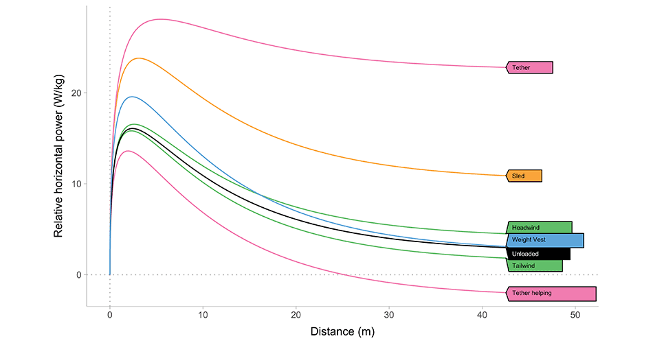
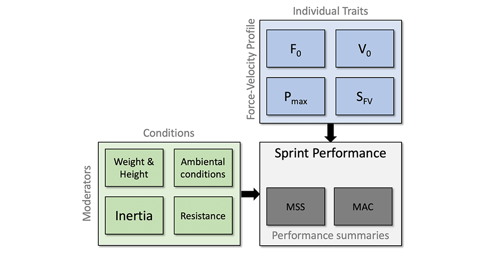
In the previous installment of this article series, we played in the theoretical sandbox assuming \(F_0\) and \(V_0\) to be causal determinants of performance, and we inspected how sprint performance (summarized with \(MSS\) and \(MAC\) parameters) changed under different load types and magnitudes. This gave us the theoretical expectations.
In this part of the article series, we will perform the analysis of both AVP and FVP using real sprinters under different load conditions. This data was collected thanks to Håkan Andersson. We originally wanted to write a research paper, but nobody wanted to write it; pun intended (well, I wrote the {shorts} package and the analysis; so understandably, I was fed up with writing). So I decided to convert my analysis workbook into blog article instead. Anyway, maybe we will/can write the article if we consider this to ne pre-print and we receive feedback, or even better, someone volunteers to write the paper about it.
Anyway, the hypothesis of the paper is made under the assumption that FVP represents causal determinant of performance (which I disagree with), which implicitly states that \(F_0\) and \(V_0\) should be the same under different resisted sprint type and load magnitude conditions. If they are not, then we cannot consider them as causal determinants of performance or traits that we uncover, but rather instrumental performance summary/aggregate (which is my opinion).
Anyway, as opposed to the scientific article, I will not provide and abstract – you will need to plow through the graphs and the analysis. I will only state that we have stumbled on something VERY INTERESTING. Keep on reading to find out what.
Methods
27 athletes presented for testing in a rested and hydrated state in their typical training attire. The body mass and height was measured before the warm-up.
An individual 45 min warm up including dynamic movements, technical drills and a 3-4 submaximal acceleration sprints up to 50m, with increasing in intensity up to 90% of self-selected maximal velocity was performed.
The Laser (Laser Speed by Ergotest Innovation) and the tether (DynaSpeed by Ergotest Innovations) was positioned 3 meters behind the starting line and the athletes was instructed to position the toes of the front foot just behind the starting line. The zero position was automatically set by the DynaSpeed and measured by the Laser Speed.
Athletes were afforded a 5min passive rest period prior to testing, while the testing procedures were explained to them. The participants who wore spiked shoes performed five maximal effort sprints from crouched starting position. The test protocol started with a 30m sprint with 32% of BM resisted with DynaSpeed followed by 16% for 40m and 8% for 40m. The athletes instant velocity was measured with DynaSpeed at 200hz.
Before the fourth sprint the athletes were loaded with a weight west weighing 8% (closest 0,5kg) of their BM. The fourth sprint was conducted with the weighted west for 40m, and the instant velocity was measured with Laser Speed at 200hz. Also, the fifth sprint (unloaded conditions) was run over 40m, and velocity measured with Laser Speed at 200hz. No random order was used during the test for practical and safety reasons. The rest period between the five trials was at least 5 minutes.
12 athletes only conducted resisted sprints with 8% of BM, 8% with weighted west and unloaded conditions following the same protocol.
All athletes participating in the study had great experience from sprint training with resistance. Every one had used sleds as resistance and a majority DynaSpeed. Only two athletes had experience from sprinting with vertical loading in the form of a weighted west.
Athlete characteristics
Athletes’ gender, number, height, and weight can be seen in the table below.
| gender | n | height | weight |
|---|---|---|---|
| F | 9 | 168.56 ± 7.25cm | 63.44 ± 8.75kg |
| M | 18 | 182.33 ± 4.38cm | 75.72 ± 7.04kg |
External load
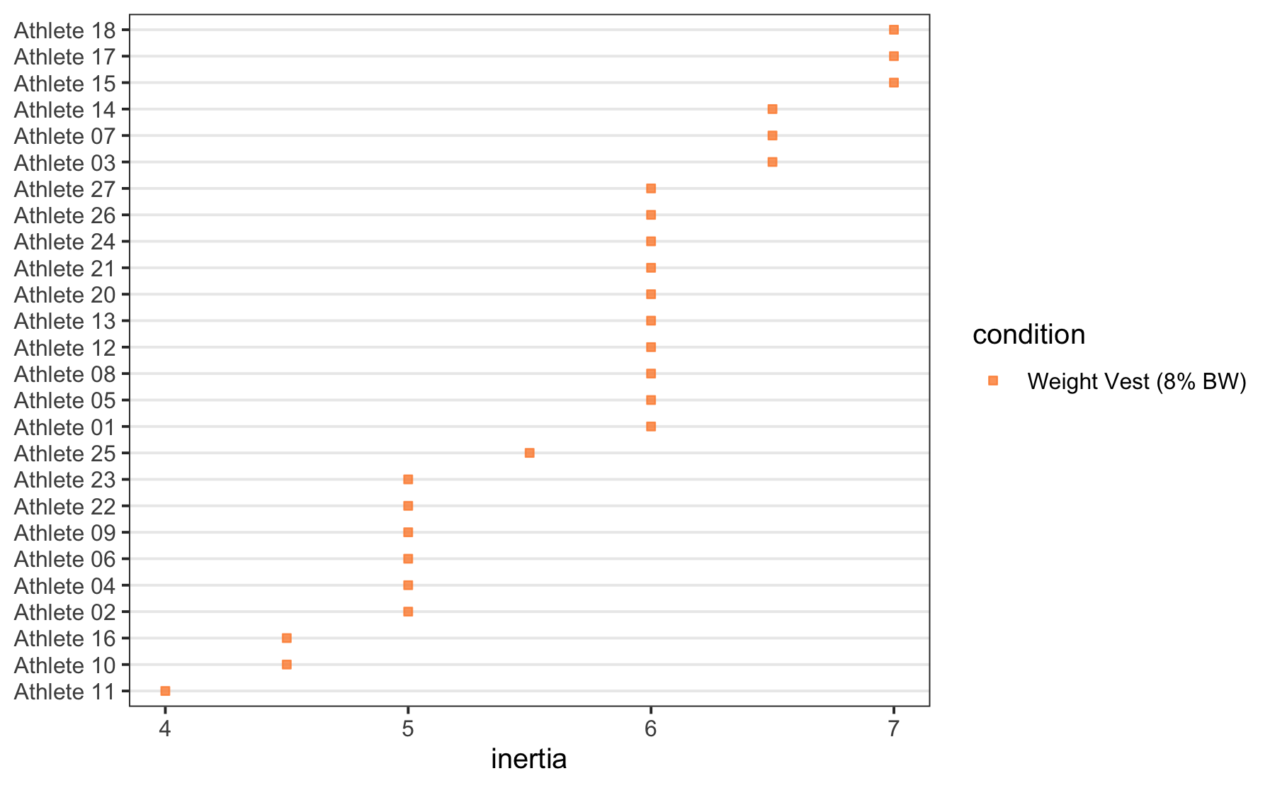
Weight vest condition represents the inertial load, where the athlete needs to accelerate additional mass horizontally. Additional air resistance due to a slightly larger body area is ignored in the calculations of forces. Figure below depicts actual load used for every athlete for the Weight Vest condition.
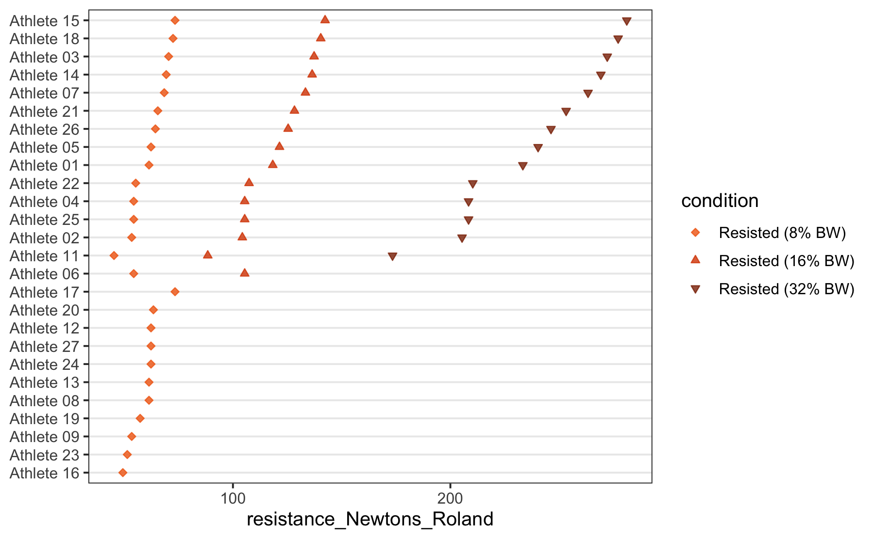
DynaSpeed resistance is selected to be 32, 16, and 8% of BW. This load represents horizontal force (without inertia, or mass). The exact force in \(Newtons\) is calculated based on the equation below (Van Den Tillaar et al. 2023), since DynaSpeed resistance is expressed in \(kilograms\):
\[
F = 3.5132 + load \times 9.99
\]
Figure below depicts actual load (i.e., force) used for every athlete for the Resisted conditions.
Model fitting
Data from the Laser and DyanSpeed was utilized to estimate short sprint parameters (i.e., \(MSS\), \(TAU\), \(MAC\), and \(PMAX\)), as well as FVP (\(F_0\), \(V_0\), peak powers), in the following approach:
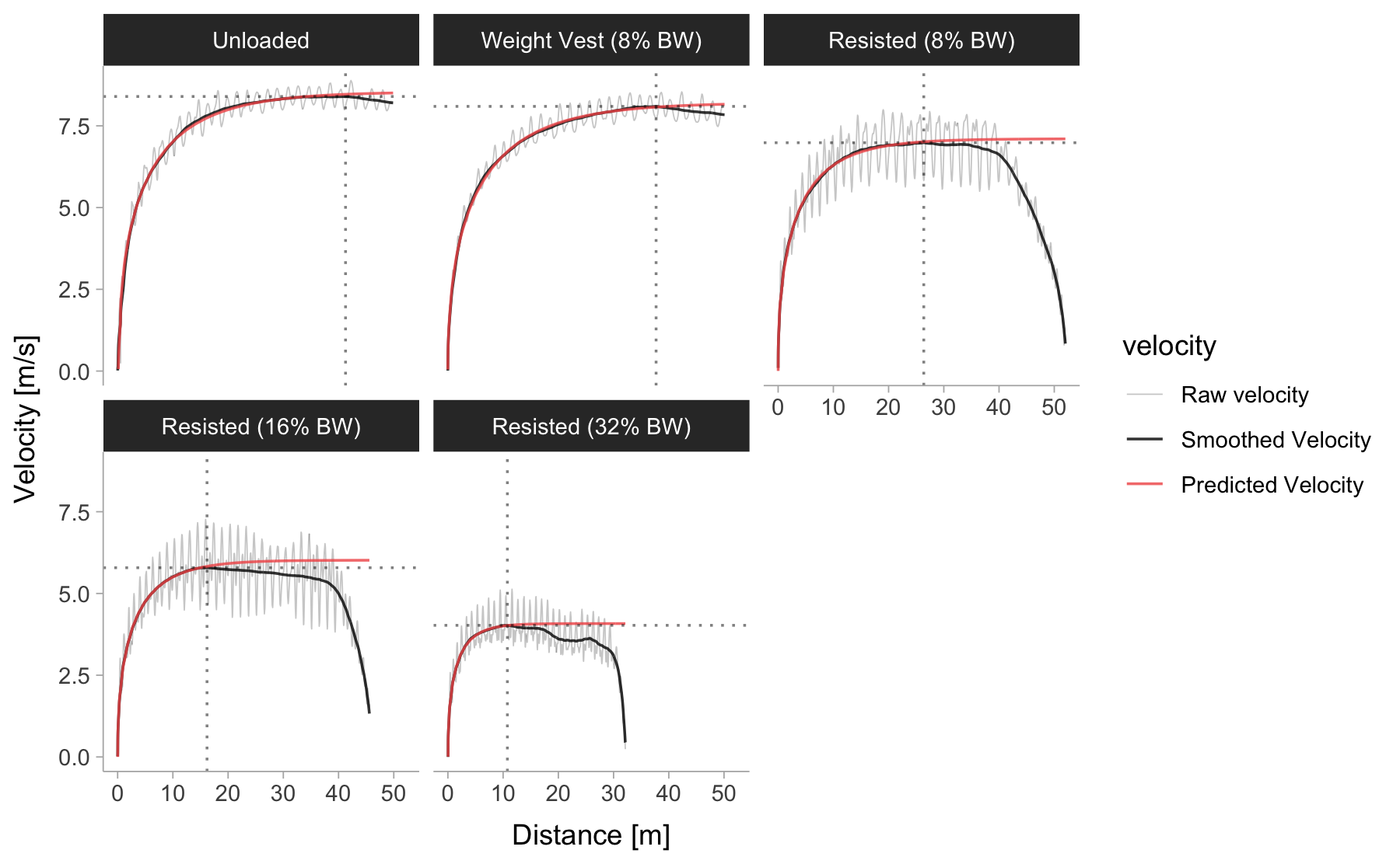
- Data was trimmed to the point of peak value in the smoothed velocity (horizontal and vertical dotted lines on the figure below)
- Data was further trimmed to only include smooth velocity over 0.5 \(ms^{-1}\). This way lag in measured velocity is not affecting estimated model parameters
- Short sprint mono-exponential model besides \(MSS\) and \(TAU\) parameters included \(TC\) (time-correction) parameter that serves the intercept function and allows the predicted velocity not to be forced to start at t = 0 \(s\) (see more here).
- Smoothed (NOT raw) velocity and time was used to estimate the MSS and TAU parameters
Figure below depicts raw and smoothed velocities across measured distance as well as predicted velocity for 5 trials using single athlete.
Please note that for Unloaded and Weight Vest conditions, Laser gun was used to provide velocity traces. For Resisted trials, DynaSpeed was used, yielding two systems of measurement. Laser and DynaSpeed demonstrated high agreement and can be thus used interchangeably (Van Den Tillaar et al. 2023).
Interesting thing to notice in the graph below is that higher variability of the instantaneous (i.e., raw) velocity around the smoothed (step-averaged) velocity happens in the resisted sprinting conditions. This implies that athletes experience higher deceleration between the steps and must produce more acceleration during the steps (i.e. while on the ground) in resisted conditions. This is not captured by this Small World model (which I discussed about here), but it could be very interesting point for discussions, but not in this article.
Force-Velocity profile for each sprint is estimated using estimated \(MSS\) and \(TAU\) parameters, inertia used (i.e., weight vest), horizontal resistance by the DynaSpeed, athlete weight and height as well as default environmental conditions to calculated air resistance (barometric pressure of 760 \(Torrs\), air temperature of 25 \(C^\circ\)). This is done using the shorts::create_FVP() function from the {shorts} package.
Results
Missing trials
Table below contains sprint trials performed by each athlete
| athlete | gender | weight | height | Resisted (32% BW) | Resisted (16% BW) | Resisted (8% BW) | Weight Vest (8% BW) | Unloaded |
|---|---|---|---|---|---|---|---|---|
| Athlete 01 | M | 72 | 181 | 31/10 13:18 |
31/10 13:32 |
31/10 13:37 |
31/10 13:50 |
31/10 14:05 |
| Athlete 02 | F | 63 | 164 | 09/11 17:45 |
09/11 17:50 |
09/11 17:55 |
09/11 18:03 |
09/11 18:10 |
| Athlete 03 | F | 84 | 172 | 01/11 09:29 |
01/11 09:37 |
01/11 09:45 |
01/11 09:59 |
01/11 10:07 |
| Athlete 04 | M | 64 | 177 | 31/10 09:26 |
31/10 09:32 |
31/10 09:37 |
31/10 09:52 |
31/10 09:46 |
| Athlete 05 | M | 74 | 183 | 09/11 16:44 |
09/11 16:51 |
09/11 16:56 |
09/11 17:08 |
09/11 17:20 |
| Athlete 06 | F | 64 | 174 | 31/10 13:20 |
31/10 13:33 |
31/10 13:45 |
31/10 14:02 |
|
| Athlete 07 | M | 81 | 187 | 09/11 16:43 |
09/11 16:50 |
09/11 16:55 |
09/11 17:05 |
09/11 17:18 |
| Athlete 08 | M | 74 | 180 | 04/11 10:12 |
04/11 10:26 |
04/11 10:30 |
||
| Athlete 09 | M | 63 | 175 | 04/11 09:05 |
04/11 09:21 |
04/11 09:36 |
||
| Athlete 10 | F | 58 | 170 | 01/11 10:03 |
01/11 10:10 |
|||
| Athlete 11 | F | 53 | 153 | 09/11 16:48 |
09/11 16:54 |
09/11 16:59 |
09/11 17:14 |
09/11 17:27 |
| Athlete 12 | M | 74 | 180 | 04/11 10:51 |
04/11 10:59 |
04/11 11:06 |
||
| Athlete 13 | M | 73 | 184 | 04/11 09:02 |
04/11 09:10 |
04/11 09:28 |
||
| Athlete 14 | M | 83 | 187 | 07/11 10:56 |
07/11 11:06 |
07/11 11:17 |
07/11 11:31 |
07/11 11:41 |
| Athlete 15 | M | 87 | 187 | 31/10 13:17 |
31/10 13:22 |
31/10 13:34 |
31/10 13:53 |
31/10 13:57 |
| Athlete 16 | F | 58 | 178 | 04/11 09:46 |
04/11 09:53 |
04/11 09:57 |
||
| Athlete 17 | M | 87 | 189 | 04/11 10:13 |
04/11 10:19 |
04/11 10:28 |
||
| Athlete 18 | M | 86 | 175 | 08/11 16:18 |
08/11 16:24 |
08/11 16:36 |
08/11 16:44 |
08/11 16:51 |
| Athlete 19 | M | 68 | 181 | 04/11 10:53 |
04/11 11:17 |
|||
| Athlete 20 | M | 75 | 180 | 04/11 10:15 |
04/11 10:22 |
04/11 10:32 |
||
| Athlete 21 | M | 78 | 183 | 31/10 09:25 |
31/10 09:31 |
31/10 09:36 |
31/10 09:44 |
31/10 09:44 |
| Athlete 22 | F | 65 | 172 | 09/11 16:45 |
09/11 16:52 |
09/11 16:57 |
09/11 17:12 |
09/11 17:25 |
| Athlete 23 | F | 60 | 165 | 04/11 09:44 |
04/11 09:51 |
04/11 09:56 |
||
| Athlete 24 | M | 74 | 179 | 04/11 09:04 |
04/11 09:13 |
04/11 09:25 |
||
| Athlete 25 | F | 66 | 169 | 09/11 17:44 |
09/11 17:50 |
09/11 17:54 |
09/11 18:00 |
09/11 18:08 |
| Athlete 26 | M | 76 | 188 | 09/11 16:46 |
09/11 16:53 |
09/11 16:58 |
09/11 17:10 |
09/11 17:23 |
| Athlete 27 | M | 74 | 186 | 04/11 10:54 |
04/11 11:01 |
Table 1: Sprint trials performed by each athlete
Individual models
Following figure depicts individual smoothed and predicted velocities. Double click on the athlete in the legend to isolate the athlete.
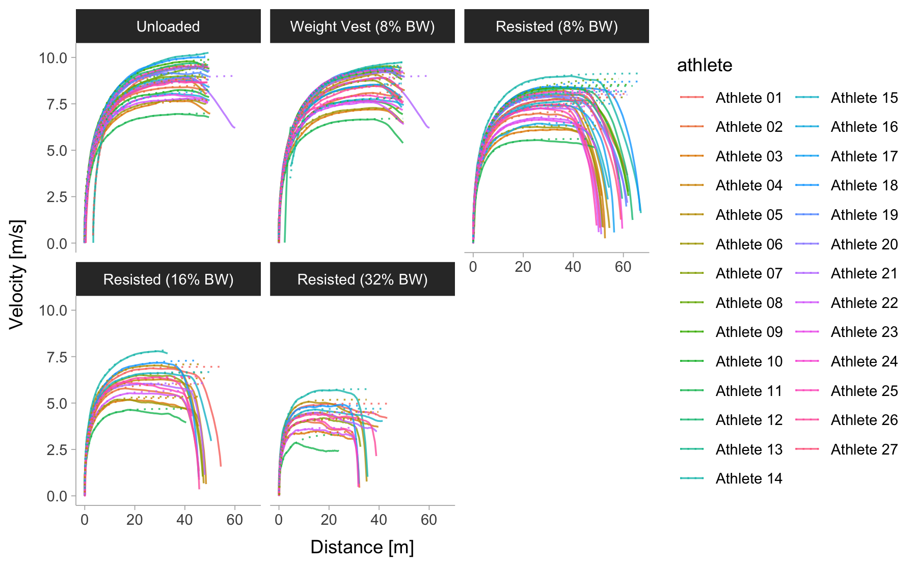
Removed athletes
The following athletes were removed from the results. You can easily see in the above figure if you select these athletes and check the velocity traces.
- Athlete 11 (Resisted 32% BW)
- Athlete 08 (Resisted 8% BW)
- Athlete 02 (Resisted 16% BW)
- Athlete 12 (Weigh Vest 8%)
Model fit metrics
The following figure depict distribution of the root-mean-squared-error (RMSE) of the model fits. The lower the number, the better the model fit.
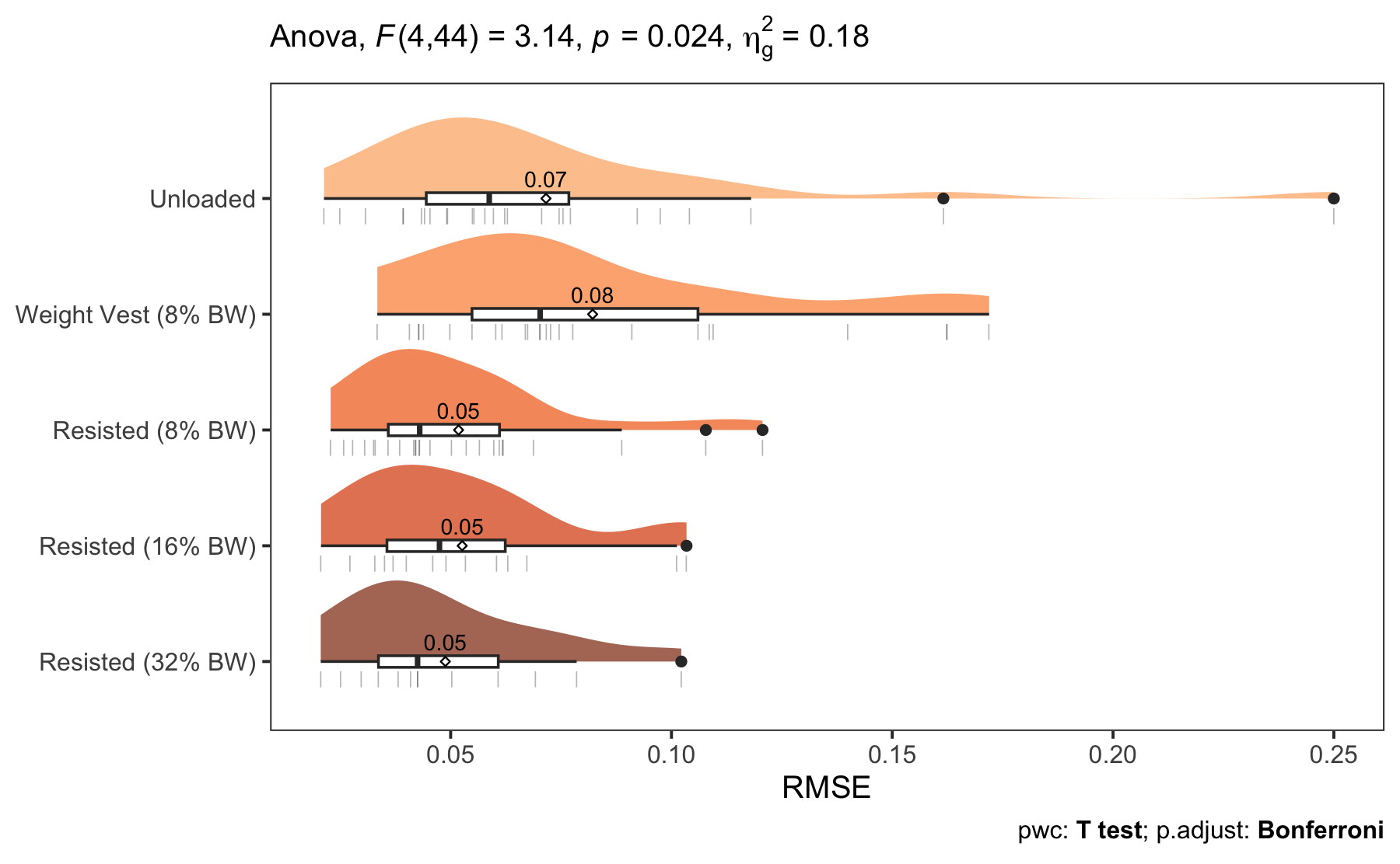
I will use this graph to compare the distribution of the estimates as well as to depict statistical inference using repeated-measured ANOVA with Bonferroni adjusted pairwise t-tests. Actually, the t-tests are performed and depicted only if the ANOVA is statistically significant (i.e., \(p<0.05\)), with the reference group being the Unloaded condition.
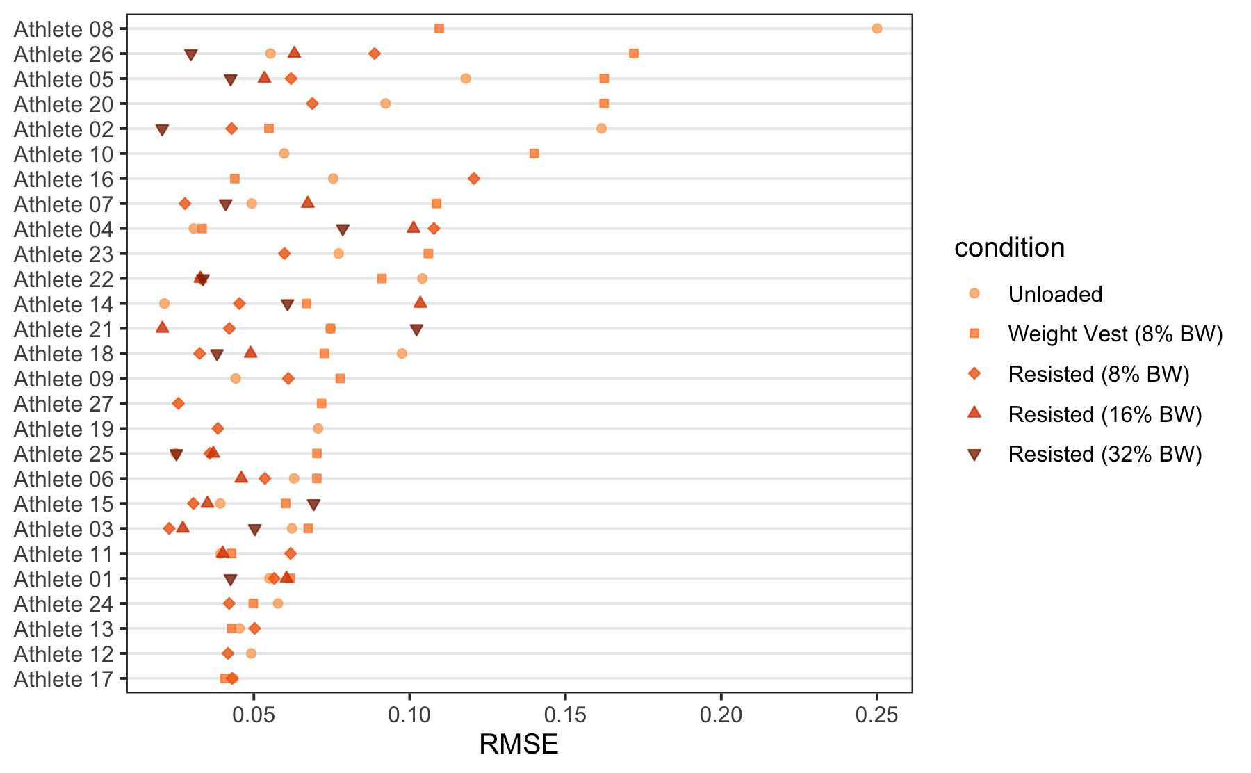
The following graph depicts individual RMSE for all sprint conditions. I will also stick to this type of graph thorough this article.
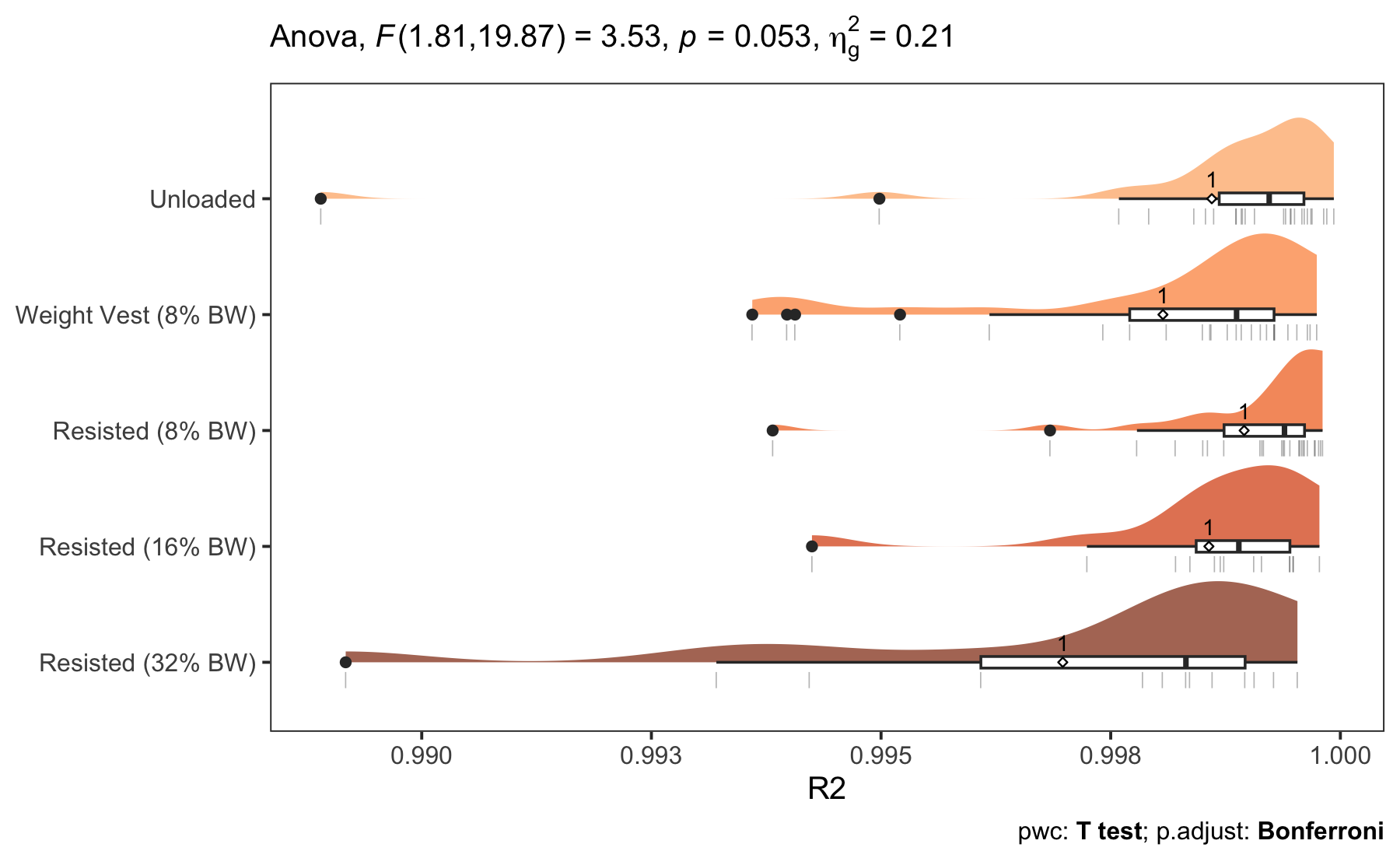
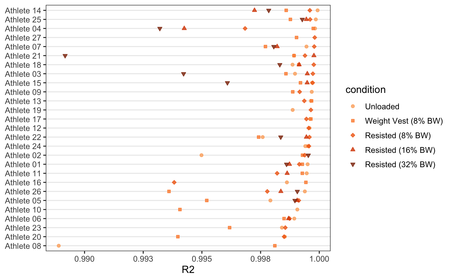
The following figures depict \(R^2\) metric. The higher the number, the better the model fit.
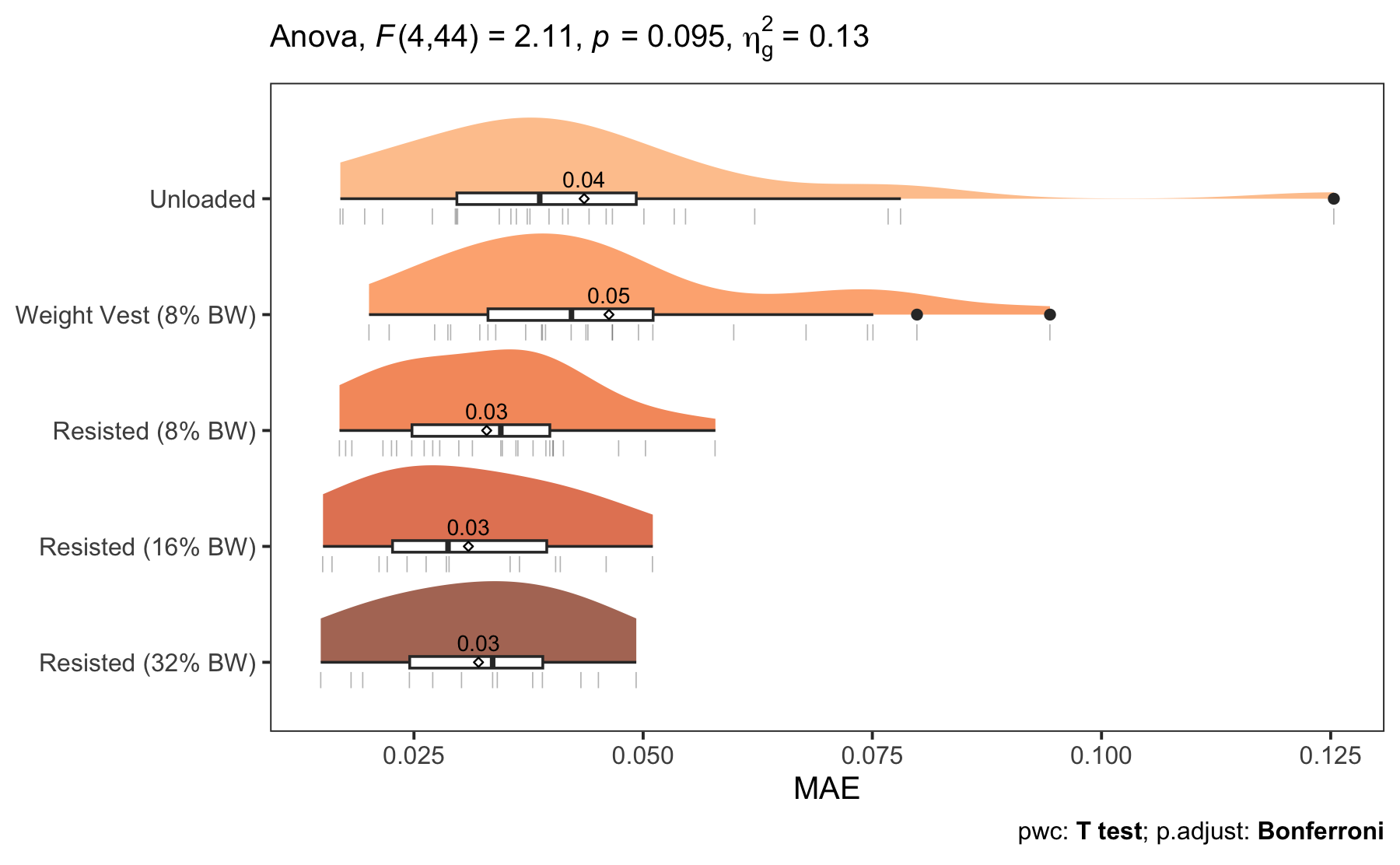
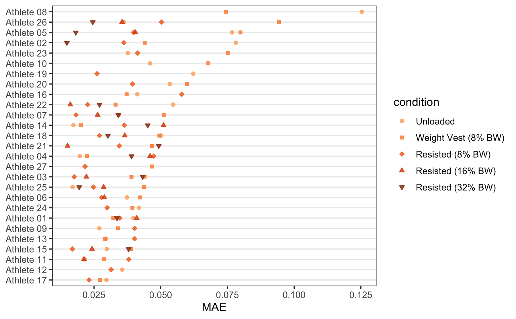
The following figures depict mean-absolute-error (MAE) of the model fits. The lower the number, the better the model fit.
And finally, figure below depicts max-absolute-error (maxAbsErr). This is the single biggest absolute difference between the observed data and model predictions (i.e., outlier). The lower the number, the better the model fit.
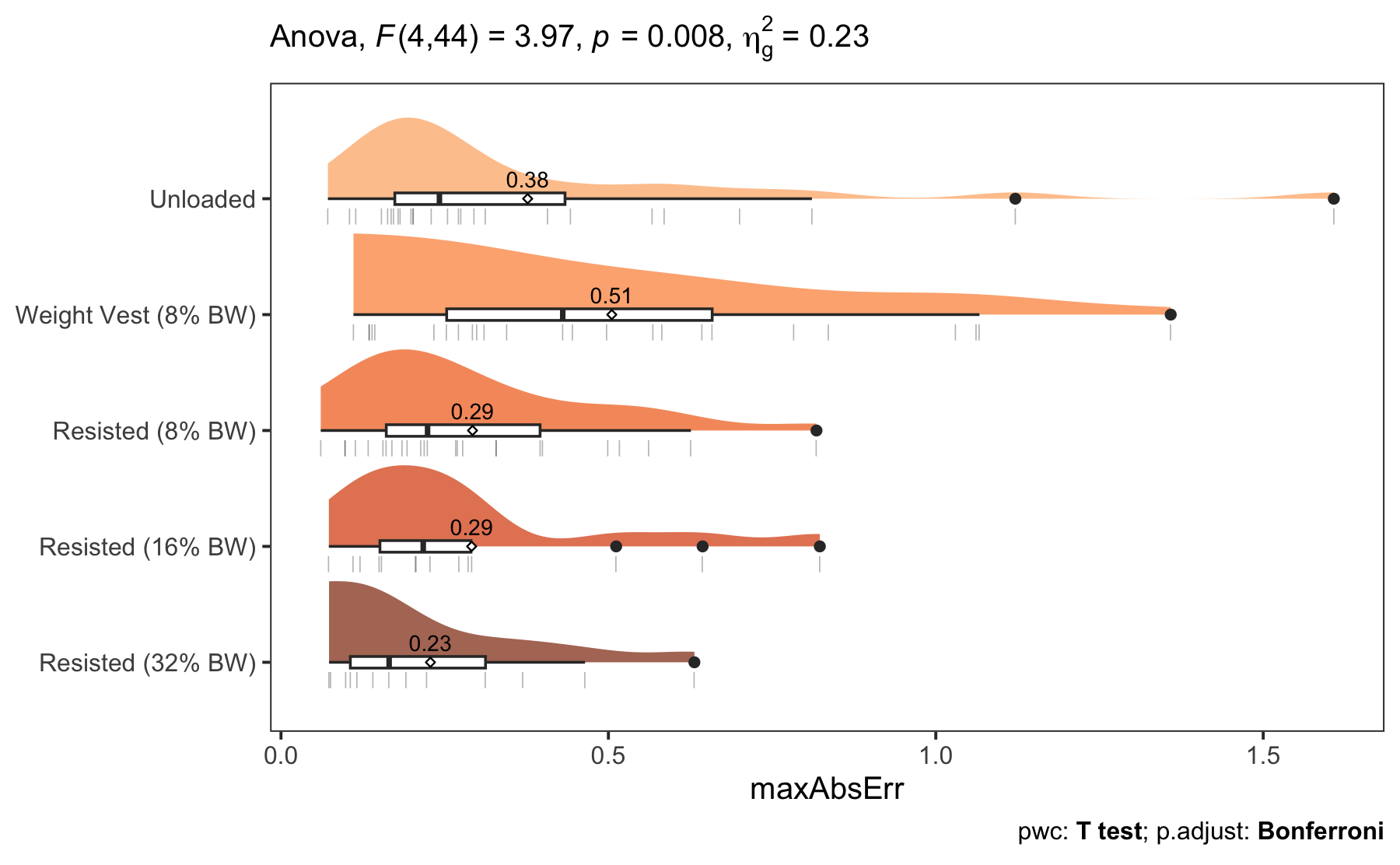
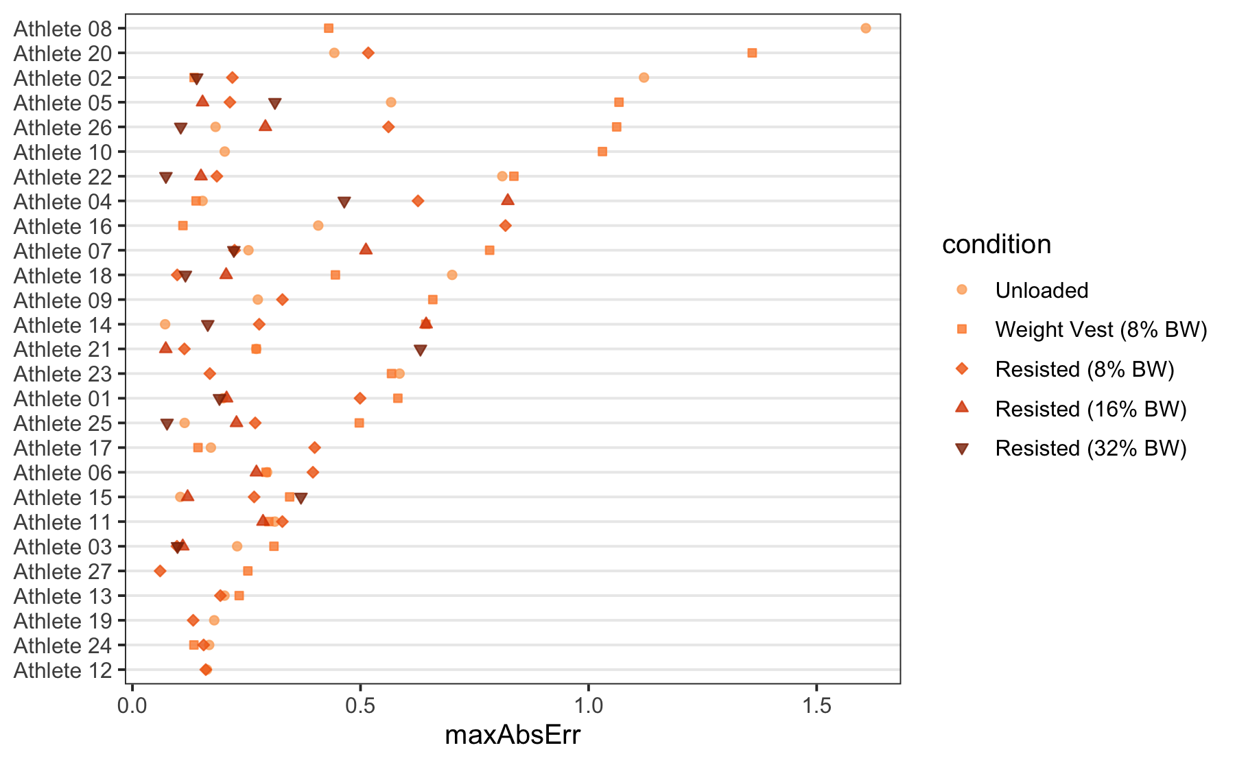
Overall, there is no statistically significant difference in any model-fit metric across sprint conditions.
Estimated \(MSS\)


Responses