Sprint Profiling – Common Problems and Solutions Part 1

Introduction

Short sprints (i.e., sprints without deceleration, usually <6sec) profiling represents a process of fitting a simple mathematical model (mono-exponential model – explained later) to the observed data with the aims of describing/summarizing, comparing, predicting, and hopefully making some intervention/causal claims. Process of model fitting, or in this case profiling, is an optimization process of finding the model parameters that best fit the data (i.e., minimize the error, most often the sum of squared errors, although other errors can be minimized). In plain English, we are making a simple (but useful) map (i.e., model) of the territory using collected data.

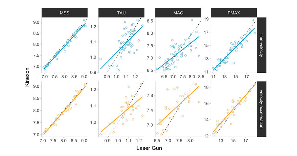
In this article I will guide you through common ways of making a map (i.e., profiling) from different types of short sprint data. This includes, but it is not limited to: (1) radar gun or laser gun data, (2) tether data (like DynaSpeed), (3) timing gates or photo cells data, and (4) GPS (like Catapult) or local positioning systems (LPS; like Kinexon) used to monitor the training sessions. All of these have some specific problems that can lead to biased and imprecise maps. I will walk you through common scenarios that you will stumble upon and provide some potential solutions that can alleviate certain problems.

We are going to do the analysis in R language (I wholeheartedly recommend installing RStudio from Posit) using the {shorts} package which you can install by running:

# Install from CRAN
install.packages("shorts")

# Or the development version from GitHub
# install.packages("remotes")
remotes::install_github("mladenjovanovic/shorts")

I recommend installing {shorts} package from GitHub, since here you can find the latest developmental version. I must note that for the code in this article to run, you will need 2.5.0.9000+ version of the {shorts} package, which is still not on CRAN by the time of this writing.

I will provide the R code for everything, and if the code is not shown just click the “Show/Hide Code” which is located over the figure or table output.

The Map

Sprint kinematics can be simply mapped-out using the mono-exponential Equation 1.

\[
v(t) = MSS \times (1 – e^{-\frac{t}{TAU}})
\tag{1}\]

The parameters in Equation 1 are the Maximum Sprinting Speed (\(MSS\)), which is measured in meters per second (\(ms^{-1}\)), and the Relative Acceleration (\(TAU\)), which is measured in seconds (\(s\)). The parameter \(TAU\) denotes the quotient obtained by dividing the \(MSS\) by the initial Maximum Acceleration (\(MAC\)), which is expressed in units of meters per second squared (\(ms^{-2}\)) and can be represented by Equation 2. It should be noted that \(TAU\) represents the duration needed to attain a velocity equivalent to 63.2% of the \(MSS\), as determined by the given Equation 1.

\[
MAC = \frac{MSS}{TAU}
\tag{2}\]

While \(TAU\) is a parameter employed in the equations and subsequently estimated, it is advisable to employ and report \(MAC\) as it is more straightforward to comprehend, particularly for professionals and trainers.

Having said that, the another form of Equation 1 that can be used as an alternative is Equation 3 in which we changed \(TAU\) for \(\frac{MSS}{TAU}\).

\[
v(t) = MSS \times (1 – e^{-\frac{t \times MAC}{MSS}})
\tag{3}\]

By performing derivation of Equation 1, we get equation for the horizontal equation (Equation 4).

\[
a(t) = \frac{MSS}{TAU} \times e^{-\frac{t}{}}
\tag{4}\]

The equation for distance covered (Equation 5) can be derived by integrating Equation 1.

\[
d(t) = MSS \times (t + TAU \times e^{-\frac{t}{TAU}}) – MSS \times TAU
\tag{5}\]

One cool feature of the mono-exponential model is the linear relationship between acceleration and velocity, making it great for profiling purposes (Equation 6).

\[
a(v) = MAC – v \times \frac{MAC}{MSS}
\tag{6}\]

All of this is easier to describe graphically. Figure 1 depicts mathematical model behavior using true parameter values for four athletes.

library(tidyverse)
library(shorts)

kinematics_df <- tribble(
  ~athlete,              ~MSS, ~MAC,
  "A (high speed, low acceleration)",   10,    6,
  "B (low speed, high acceleration)",  7,    9,
  "C (low speed, low acceleration)",   7,    6,
  "D (high speed, high acceleration)", 10,   9
) %>%
  group_by(athlete) %>%
  reframe(predict_kinematics(MSS = MSS, MAC = MAC, max_time = 20, frequency = 10)) %>%
  ungroup()

# Time velocity
gg1 <- kinematics_df %>%
  filter(time <= 10) %>%
  ggplot(aes(x = time, y = velocity, color = athlete)) +
  geom_line() +
  xlab("Time (s)") +
  ylab("Velocity (m/s)") +
  theme(legend.position = c(0.6, 0.4)) +
  scale_x_continuous(expand = c(0, 0), limits = c(0, NA)) +
  scale_y_continuous(expand = c(0, 0), limits = c(0, NA)) 

gg1

# Distance velocity
gg2 <- kinematics_df %>%
  filter(distance <= 50) %>%
  ggplot(aes(x = distance, y = velocity, color = athlete)) +
  geom_line()  +
  xlab("Distance (m)") +
  ylab("Velocity (m/s)") +
  theme(legend.position = c(0.6, 0.4)) +
  scale_x_continuous(expand = c(0, 0), limits = c(0, NA)) +
  scale_y_continuous(expand = c(0, 0), limits = c(0, NA)) 

gg2

# Acceleration - time
gg3 <- kinematics_df %>%
  filter(time <= 10) %>%
  ggplot(aes(x = time, y = acceleration, color = athlete)) +
  geom_line() +
  xlab("Time (s)") +
  ylab("Acceleration (m/s/s)") +
  theme(legend.position = c(0.6, 0.4)) +
  scale_x_continuous(expand = c(0, 0), limits = c(0, NA)) +
  scale_y_continuous(expand = c(0, 0), limits = c(0, NA)) 

gg3

# Acceleration - distance
gg4 <- kinematics_df %>%
  filter(distance <= 50) %>%
  ggplot(aes(x = distance, y = acceleration, color = athlete)) +
  geom_line() +
  xlab("Distance (m)") +
  ylab("Acceleration (m/s/s)") +
  theme(legend.position = c(0.6, 0.4)) +
  scale_x_continuous(expand = c(0, 0), limits = c(0, NA)) +
  scale_y_continuous(expand = c(0, 0), limits = c(0, NA)) 

gg4

# Distance - time
gg5 <- kinematics_df %>%
  filter(distance <= 50) %>%
  ggplot(aes(x = distance, y = time, color = athlete)) +
  geom_line() +
  xlab("Distance (m)") +
  ylab("Time (s)") +
  theme(legend.position = c(0.8, 0.3)) +
  scale_x_continuous(expand = c(0, 0), limits = c(0, NA)) +
  scale_y_continuous(expand = c(0, 0), limits = c(0, NA)) 

gg5

gg6 <- kinematics_df %>%
  ggplot(aes(x = velocity, y = acceleration, color = athlete)) +
  geom_line() +
  xlab("Velocity (m/s)") +
  ylab("Acceleration (m/s/s)") +
  theme(legend.position = c(0.7, 0.8)) +
  scale_x_continuous(expand = c(0, 0), limits = c(0, NA)) +
  scale_y_continuous(expand = c(0, 0), limits = c(0, NA)) 

gg6

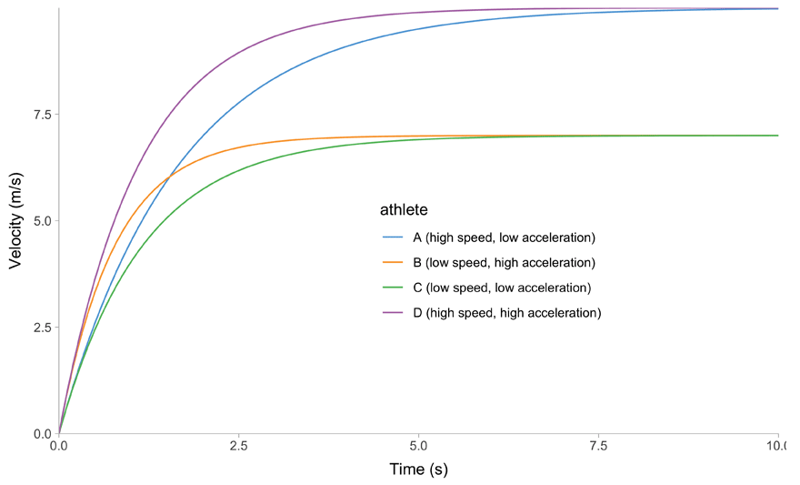
(a) Time~Velocity trace

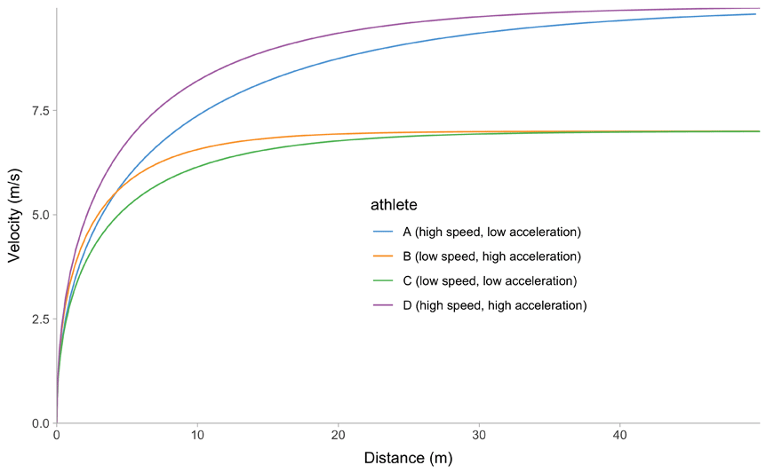
(b) Distance~Velocity trace

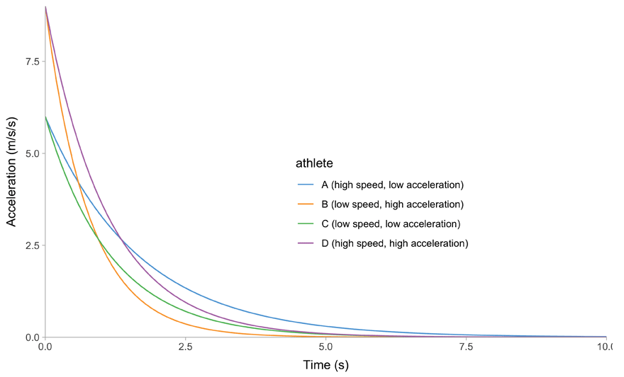
(c) Time~Acceleration trace

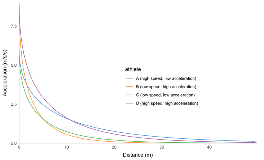
(d) Distance~Acceleration trace

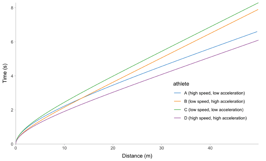
(e) Distace~Time trace

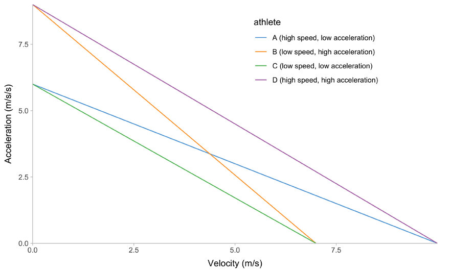
(f) Velocity~Acceleration trace

Figure 1: Kinematics of the mono-exponential model using four hypothetical athletes

Once we have the model parameters, we can estimate (i.e., predict) various model kinematic behavior. If we know the weight and height of the athlete, as well as air conditions (pressure, temperature, and wind), we can add into the mix another model to calculate air resistance and get kinetics, or forces, power, and work values. With forces being known, we can estimate Force-Velocity Profile (FVP). This is a topic for another article. In this one we will stick to the simple mono-exponential model and \(MSS\) and \(MAC\) parameters, since if we cannot estimate them correctly, we will propagate the errors to all other predictions which depend on their valid and precise estimation. In plain English again, if you suck at estimating \(MAC\) or \(MSS\), then the FVP will be shit as well. So let us focus on this task first, and worry about fancy FVP later (or in another article).

Due to it’s elegant linear relationship between acceleration and velocity (Figure 1 (f)), we can also call mono-exponential model a Acceleration-Velocity Profile, or AVP. So, when we estimate the AVP, we estimate the \(MSS\) and \(MAC\) parameters using the mono-exponential model.

Why is this better than looking at the raw data?

My Devil’s advocate nature motivates me that in a room full of coaches, I will defend “theory and sports science” (I will defend the nerds), and in the room full of “evidence-based lab-coats”, I will defend practice and coaches (I will defend the jocks). So let me clearly state that this map (i.e., AVP and FVP with it) will NOT make you a better coach. Just by simply profiling someone, you will not magically uncover some sprinting Holy Grail which will make your athletes faster, nor will you know how and where to intervene in the Large World (i.e., territory) based on the sensitivity analysis of the map/model (i.e., playing with whether increasing \(MSS\) or \(MAC\) parameter will yield faster split times for a given individual). You might think you know where to intervene, but that’s just characteristic of the map, not the territory (and this is often forgotten, unfortunately).

In short, this is a tool, not the Truth. But models can be very useful. For example, some experienced coaches can glance at the split times and know who is good accelerator and who has the high top speed. But this model makes this far easier and more elegant since it summarizes or aggregates the short sprint performance into only two parameters. Here is an example of split times over 5, 10, 20, 30, and 40-meters for two athletes:

• 1.45, 2.23, 3.59, 4.88, 6.14 seconds
• 1.51, 2.28, 3.58, 4.77, 5.92 seconds

By looking at these split times, what can you convey? Hard, isn’t it? But what if I tell you that these were generated using \(MSS\) of 8 \(ms^{-1}\) and \(MAC\) of 7 \(ms^{-2}\) for the first athlete and \(MSS\) of 9 \(ms^{-1}\) and \(MAC\) of 6 \(ms^{-2}\) for the second.

So, rather than scratching your head looking at time-velocity trace, or split times, one can simply glance at \(MSS\) and \(MAC\) parameters and have some insight into the characteristic behavior. It is slippery slope to call these traits or characteristics of the athlete, e.g., acceleration and max speed characteristic/trait/quality of an individual, but from a pragmatist position they are still useful in zipping (or compressing) the data into two parameters. Yes, athletes with higher \(MAC\) will have higher acceleration, but I will nitpick and restrain over calling \(MAC\) (or \(MSS\)) a trait, since these are the parameters of the Small World model, and traits can be considered attributes of the Large World. So be very cautious when jumping this is/ought gap. For more discussion on this topic check my Circular Performance Model article.

Thus, it is important to keep beating the dead horse with “map is not the territory” and “tools, not truths”, since people tend to forget these.

Glad that we have this important philosophical discussion off the table and we can move to more practical stuff of parameter estimation (i.e., profiling).

Model parameters estimation

So far we have explored the kinematics behavior of the simple mono-exponential model using the known \(MSS\) and \(MAC\) parameters. What we can do with “modelling”, “fitting” or “profiling” is to estimate the parameters that give the best fit to the observed data. This can be done in numerous ways, using computation or analytic solutions. Long story short, the computer tries various combinations of \(MSS\) and \(MAC\) and checks which one minimizes the residuals (i.e., difference between observed and fitted values) and their summary metric (usually sum of squared errors; for more info check the FREE online version of the bmbstats book (Jovanović 2020)). For our model, this is done using the non-linear regression (except for the velocity~acceleration trace, where we can use simple linear regression, but more about it later).

So in essence, when we use model fitting using the observed data, we tell the computer: “Look buddy, this is the data I have. Find the model parameters that best fit the observed data”. But as you will soon find out, this can result in biased estimates (and we can know this by simulating the observed data using known parameter values, then check how good are we in recovering their true values; for example see Jovanović (2023)).

What will follow next is model fitting (i.e., estimating \(MSS\) and \(MAC\) parameters) using different types of data, problems that you might stumble upon, and potential solutions.

Laser/Radar Gun or the analysis of the time-velocity trace

Let’s start with a perfect example and then add weirdness as we go. Usually, the radar guns or laser guns, such as LaserSpeed by MuscleLab, provide high frequency velocity of certain body position (most often the low back, which we take as the proxy to center-of-mass or COM). This velocity will fluctuate due to inherent acceleration and deceleration during stride cycle, as well as body-movement or shifting. Most systems provide some type of smoothed velocity, which we can think of as a stride-average velocity. Figure 2 depicts a simulated example using known \(MAC\) equal to 6 \(ms^{-2}\) and \(MSS\) equal to 8 \(ms^{-1}\). Figure 2 (a) depicts true model (i.e., stride-average velocity) as a black line and raw velocity (i.e., velocity of low back) as thin black line. This is of course simply simulated by adding sinusoidal waves and random error around the true velocity.

Figure 2 (b) depict the same data as Figure 2 (a), but adds smoother on top (depicted as thick transparent blue line). There are multiple ways to create smoothed velocity, and here I have used loess() or local polynomial regression fitting (LOESS; YouTube video) which uses the raw velocity, but as you can see it is pretty close to the true velocity. Then why not stick to the smoother then? Well, the problem is that the parameters estimated by this or any other smoother do not have theory-backing like our AVP or mono-exponential model. In other words, the parameters of the smoother mean jack shit (i.e., they are called non-parametric for a reason). But in a few moments you will see how we can still use them.

Laser or Radar gun manufacturers often provide both velocities in their output (i.e., raw and smoothed), but often the exact smoothing method is either unknown or represents proprietary secret.

My Devil’s advocate nature motivates me that in a room full of coaches, I will defend “theory and sports science” (I will defend the nerds), and in the room full of “evidence-based lab-coats”, I will defend practice and coaches (I will defend the jocks). So let me clearly state that this…