How to Analyze Movement Screen Tests?
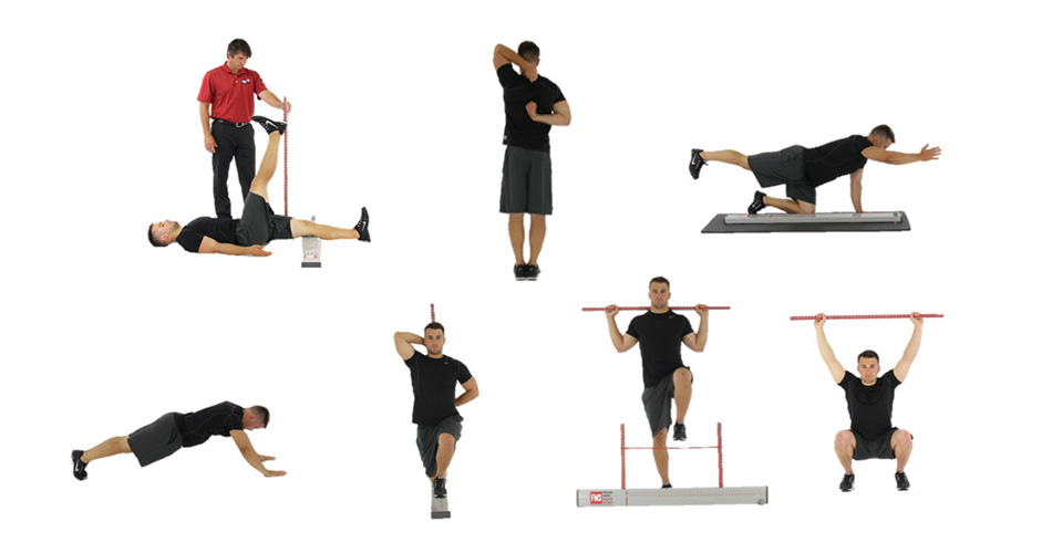
In the recent post I shared the movement screen we designed and implemented. The question now is how to analyze the data and make real life decisions on it?
What do we need to get from the analysis in the first place? In my (current) opinion we need these:
- Identify groups of athletes with similar problems/issues
- Identify latent factors behind the movement screen
Both of them are related to identifying the buckets in movement screen. Even if we managed to get individualized plans for each athlete screened, most of them will fall into a bucket (e.g. lack of mobility, lack of control, etc). We need to identify those buckets (group of athletes with similar issues).
The bucket issue with second task is identifying the underlying factors behind the movement screen. We might have a bunch of tests, but we are interested what factors or qualities those tests evaluate. This is done with Exploratory Factor Analysis (EFA) and Principal Component Analysis (PCA). To be honest I am just starting to learn about these two and will come back to this type analysis (and this task) in near future.
We will focus on identifying the athletes with similar problems. The “problem” will be that we will not know what those problems are (for that we would need PCA/EFA) – hence we need to dig into the tests manually or use our experience (until we learn PCA/EFA).
The short summary of the Buckets Analysis™ in Team Sports:
From a movement screen tests (or any other in team sports) we should identify athletes with similar problems (task 1) and define those problems (task 2)
The task 2 is solved using PCA/EFA. The task of putting the athletes in buckets of similarity is solved with Clustering. Clustering, or K-means clustering is a machine learning algorithm that figure outs similarities between athletes and put them into a bucket (watch the great video by Jeff Leek from Coursera Course HERE).
So let’s start playing with Clustering. I have uploaded the results of Movement Screen in a CSV on the Complementary Training website.
# Load the Movement Screen Data
movementScreenData <- read.table("http://complementarytraining.com/wp-content/uploads/2014/04/Functional-Screening.csv",
    header = TRUE, sep = ",")
Here is how the data looks like
str(movementScreenData)
## 'data.frame':    27 obs. of  44 variables:
##  $ Age                    : int  27 32 26 26 24 20 23 35 30 33 ...
##  $ Weight                 : num  75 79.2 77.1 93.1 77 78.9 79 67 81.2 77.2 ...
##  $ Height                 : num  181 183 184 196 179 ...
##  $ Body.Fat               : num  0.1 0.11 0.08 0.13 0.1 0.1 0.11 0.11 0.12 0.14 ...
##  $ LBM                    : num  67.4 70.4 70.8 81.2 69 ...
##  $ BMI                    : num  22.9 23.6 22.8 24.4 24 ...
##  $ Limb.Length            : num  93 95 95 104 94 ...
##  $ Dominance              : Factor w/ 2 levels "Left","Right": 2 2 2 2 2 2 1 2 2 2 ...
##  $ Thomas.Thigh.LEFT      : int  4 4 5 3 5 4 3 4 5 3 ...
##  $ Thomas.Thigh.RIGHT     : int  4 4 5 4 5 4 4 4 5 3 ...
##  $ Thomas.Knee.LEFT       : int  3 1 4 3 4 3 4 2 4 3 ...
##  $ Thomas.Knee.RIGHT      : int  3 2 4 3 3 3 4 3 4 3 ...
##  $ Thomas.Aligment.LEFT   : int  2 5 5 5 5 5 4 5 4 5 ...
##  $ Thomas.Aligment.RIGHT  : int  2 3 5 4 5 5 3 5 5 5 ...
##  $ Internal.Rotation.LEFT : int  4 1 3 3 4 2 2 3 3 2 ...
##  $ Internal.Rotation.RIGHT: int  2 1 3 2 4 2 2 3 2 2 ...
##  $ External.Rotation.LEFT : int  3 3 4 5 3 5 5 2 3 3 ...
##  $ External.Rotation.RIGHT: int  5 4 5 5 4 5 5 2 2 2 ...
##  $ Leg.Lower              : int  3 2 3 3 3 3 2 3 3 1 ...
##  $ Diagonal.Lift          : int  3 2 3 3 3 2 3 3 3 2 ...
##  $ Sit.Up.Hold            : int  5 5 5 5 5 5 5 5 4 3 ...
##  $ Extension.Hold         : int  5 5 5 5 5 5 5 5 5 5 ...
##  $ Hamstring.LEFT         : int  3 3 4 4 4 3 4 5 4 4 ...
##  $ Hamstring.RIGHT        : int  3 3 4 4 3 3 4 5 4 5 ...
##  $ Adductor.Spread        : int  135 150 143 170 161 149 159 137 161 155 ...
##  $ Adductor.Ratio         : num  1.45 1.58 1.51 1.64 1.71 1.67 1.71 1.63 1.61 1.68 ...
##  $ Adductor.Score         : int  2 3 3 4 4 4 4 4 4 4 ...
##  $ Ankle.LEFT.distance    : int  12 11 12 16 12 6 8 11 12 10 ...
##  $ Ankle.LEFT.score       : int  4 4 4 5 4 2 3 4 4 4 ...
##  $ Ankle.RIGHT.distance   : int  11 12 12 13 10 8 11 10 10 8 ...
##  $ Ankle.RIGHT.score      : int  4 4 4 5 4 3 4 4 4 3 ...
##  $ Stork.LEFT             : int  3 3 3 2 3 2 1 2 2 1 ...
##  $ Stork.RIGHT            : int  3 2 3 2 3 2 2 2 2 1 ...
##  $ Overhead.Squat.Thighs  : int  4 4 5 4 3 5 4 4 4 4 ...
##  $ Overhead.Squat.Arms    : int  5 3 4 5 4 5 5 3 1 3 ...
##  $ Landing.LEFT           : int  2 3 2 3 3 2 2 2 2 2 ...
##  $ Landing.RIGHT          : int  1 3 3 2 3 2 3 2 3 2 ...
##  $ Landing.DOUBLE         : int  3 2 3 3 2 3 2 3 3 3 ...
##  $ Push.up.Hold           : int  3 5 5 5 4 4 5 4 0 3 ...
##  $ Lunge.LEFT             : int  3 3 3 3 3 3 3 3 3 2 ...
##  $ Lunge.RIGHT            : int  3 2 3 3 3 3 3 3 3 2 ...
##  $ Row.Hold               : int  4 5 4 3 4 4 3 2 0 4 ...
##  $ Side.Bridge.LEFT       : int  5 5 4 5 5 5 5 5 4 4 ...
##  $ Side.Bridge.RIGHT      : int  5 5 5 5 5 5 5 4 5 4 ...
Hopefully you understand how important is to make sense of this data.
What we are going to do first, before we perform K-Means Clustering is to name the players and fix the Dominance column from vector to a number
library(randomNames)

# Add some random names to the rows to represent Athletes
rownames(movementScreenData) <- randomNames(nrow(movementScreenData))

# Change Dominance factor to number
movementScreenData$Dominance <- as.numeric(movementScreenData$Dominance)
What we need to do next before performing K-Mean clustering is to normalize the data. What this basically mean is that if we have metrics of different scales (e.g. height and weight) we need to normalize them to be comparable. If we have height of 180-200cm and Thomas Test score of 1-5, guess which one will bias the clustering more? Exactly for that reason we need to normalize the score.
The simples and most used normalization is Z-Score. We will do it with build in function scale
movementScreenData <- scale(movementScreenData)
movementScreenData <- as.data.frame(movementScreenData)
And check the data now
str(movementScreenData)
## 'data.frame':    27 obs. of  44 variables:
##  $ Age                    : num  0.2359 1.1723 0.0486 0.0486 -0.326 ...
##  $ Weight                 : num  -0.3732 0.2121 -0.0805 2.1493 -0.0945 ...
##  $ Height                 : num  -0.0373 0.2728 0.4279 2.2112 -0.3475 ...
##  $ Body.Fat               : num  -0.039 0.487 -1.092 1.54 -0.039 ...
##  $ LBM                    : num  -0.4288 0.0949 0.1787 2.0206 -0.1527 ...
##  $ BMI                    : num  -0.533 0.025 -0.621 0.546 0.304 ...
##  $ Limb.Length            : num  -0.128 0.332 0.332 2.287 0.102 ...
##  $ Dominance              : num  0.347 0.347 0.347 0.347 0.347 ...
##  $ Thomas.Thigh.LEFT      : num  0.159 0.159 1.592 -1.274 1.592 ...
##  $ Thomas.Thigh.RIGHT     : num  0 0 1.36 0 1.36 ...
##  $ Thomas.Knee.LEFT       : num  -0.333 -2.333 0.667 -0.333 0.667 ...
##  $ Thomas.Knee.RIGHT      : num  -0.537 -2.15 1.075 -0.537 -0.537 ...
##  $ Thomas.Aligment.LEFT   : num  -2.923 0.611 0.611 0.611 0.611 ...
##  $ Thomas.Aligment.RIGHT  : num  -3.053 -1.804 0.694 -0.555 0.694 ...
##  $ Internal.Rotation.LEFT : num  1.2292 -2.2041 0.0848 0.0848 1.2292 ...
##  $ Internal.Rotation.RIGHT: num  -0.382 -1.672 0.908 -0.382 2.197 ...
##  $ External.Rotation.LEFT : num  -0.549 -0.549 0.439 1.426 -0.549 ...
##  $ External.Rotation.RIGHT: num  1.24 0.31 1.24 1.24 0.31 ...
##  $ Leg.Lower              : num  0.641 -0.932 0.641 0.641 0.641 ...
##  $ Diagonal.Lift          : num  0.946 -1.018 0.946 0.946 0.946 ...
##  $ Sit.Up.Hold            : num  0.539 0.539 0.539 0.539 0.539 ...
##  $ Extension.Hold         : num  0.278 0.278 0.278 0.278 0.278 ...
##  $ Hamstring.LEFT         : num  -0.343 -0.343 0.583 0.583 0.583 ...
##  $ Hamstring.RIGHT        : num  -0.667 -0.667 0.459 0.459 -0.667 ...
##  $ Adductor.Spread        : num  -1.00074 0.00497 -0.46436 1.3459 0.74248 ...
##  $ Adductor.Ratio         : num  -1.124 -0.159 -0.679 0.286 0.805 ...
##  $ Adductor.Score         : num  -1.193 -0.322 -0.322 0.548 0.548 ...
##  $ Ankle.LEFT.distance    : num  0.3014 -0.0685 0.3014 1.7808 0.3014 ...
##  $ Ankle.LEFT.score       : num  0.156 0.156 0.156 1.21 0.156 ...
##  $ Ankle.RIGHT.distance   : num  0.248 0.666 0.666 1.085 -0.17 ...
##  $ Ankle.RIGHT.score      : num  0.238 0.238 0.238 1.309 0.238 ...
##  $ Stork.LEFT             : num  1.0596 1.0596 1.0596 -0.0848 1.0596 ...
##  $ Stork.RIGHT            : num  1.041 -0.181 1.041 -0.181 1.041 ...
##  $ Overhead.Squat.Thighs  : num  -0.171 -0.171 0.986 -0.171 -1.329 ...
##  $ Overhead.Squat.Arms    : num  1.09 -0.694 0.198 1.09 0.198 ...
##  $ Landing.LEFT           : num  -0.298 1.309 -0.298 1.309 1.309 ...
##  $ Landing.RIGHT          : num  -1.491 1.107 1.107 -0.192 1.107 ...
##  $ Landing.DOUBLE         : num  0.641 -0.932 0.641 0.641 -0.932 ...
##  $ Push.up.Hold           : num  -0.656 0.955 0.955 0.955 0.149 ...
##  $ Lunge.LEFT             : num  0.192 0.192 0.192 0.192 0.192 ...
##  $ Lunge.RIGHT            : num  0.347 -2.776 0.347 0.347 0.347 ...
##  $ Row.Hold               : num  0.7463 1.4412 0.7463 0.0515 0.7463 ...
##  $ Side.Bridge.LEFT       : num  0.539 0.539 -0.916 0.539 0.539 ...
##  $ Side.Bridge.RIGHT      : num  0.639 0.639 0.639 0.639 0.639 ...
The next step is to perform Clustering. What we need to know is how many cluster we need to identify. In my opinion we can solve that question in multiple ways:
- How many qualities/factors are identified by PCA/EFA? If we know we have factors such as Lower Body Mobility, Upper Body Mobility, Landing, Core Stability, etc, maybe we should use that number
- How many resources we have? How many coaches, how much room in the gym so we can serve those groups?
- We can find out optimal number of clusters by using different algorithms
For now I will chose two, three, four and five clusters and see which one is the best fit
require(useful, quietly = TRUE)

set.seed(10)

movementScreenData.K2 <- kmeans(x = movementScreenData, centers = 2)
movementScreenData.K3 <- kmeans(x = movementScreenData, centers = 3)
movementScreenData.K4 <- kmeans(x = movementScreenData, centers = 4)
movementScreenData.K5 <- kmeans(x = movementScreenData, centers = 5)
The output of the clustering involve size of the clusters, the cluster mean for each column, the cluster membership for each row and similarity measures. To make it less confusing we will plot it.
require(gridExtra, quietly = TRUE)

K2.Clusters <- plot(movementScreenData.K2, data = movementScreenData, title = "Two Clusters")
K3.Clusters <- plot(movementScreenData.K3, data = movementScreenData, title = "Three Clusters")
K4.Clusters <- plot(movementScreenData.K4, data = movementScreenData, title = "Four Clusters")
K5.Clusters <- plot(movementScreenData.K5, data = movementScreenData, title = "Five Clusters")

grid.arrange(K2.Clusters, K3.Clusters, K4.Clusters, K5.Clusters, ncol = 2)
Each dot represent one athlete. As we can see they are not clustering perfectly. What seems like the most logical cluster number is 4 (someone please correct me if I am wrong)
Before we try with different number of clusters here is the list of athletes in each cluster (or bucket) when we performed the analysis with 4 cluster
library(xtable)

athletes.buckets <- data.frame(Name = names(movementScreenData.K4$cluster),
    Bucket = movementScreenData.K4$cluster)

# Remove the row names
row.names(athletes.buckets) <- NULL

# Print the table
print(xtable(athletes.buckets, digits = 2), type = "html")
| Name | Bucket | |
|---|---|---|
| 1 | Vigil Sandoval, Ashley | 3 |
| 2 | Trumpore, Gabriela | 1 |
| 3 | Haddenham, Stephanie | 2 |
| 4 | Archuleta, Cameron | 1 |
| 5 | Oliva, Haile | 2 |
| 6 | Alfandi, Adan | 2 |
| 7 | Rodriguez, Morgan | 1 |
| 8 | Martinez, Kellie | 2 |
| 9 | Crowe, Aaron | 4 |
| 10 | Li, Isidro | 1 |
| 11 | Marquez, Ashley | 2 |
| 12 | Sanchez-Chavez, Daryl | 2 |
| 13 | Sauls, Anthony | 1 |
| 14 | Jordan, Michael | 3 |
| 15 | Cade, Christina | 4 |
| 16 | Han, Kenny | 2 |
| 17 | Sherer, Manuel | 1 |
| 18 | Black, Oswald | 2 |
| 19 | Vue, Marcus | 1 |
| 20 | Johnson, Laurencita | 2 |
| 21 | Klose, Alexander | 4 |
| 22 | Magill, Michaellee | 1 |
| 23 | Johnson, Santos | 2 |
| 24 | Martinez-Montenegro, Erasmo | 3 |
| 25 | Chamberlain, Samantha | 4 |
| 26 | Marin, Josiah | 2 |
| 27 | Gutierrez, Hunter | 3 |
The next step is to try to figure out the number of clusters that best suits our data. For that we can use NbClust package or using FitKMeans function.
best.fit <- FitKMeans(movementScreenData, max.clusters = 10, nstart = 25)

PlotHartigan(best.fit)
I believe that the models with different clusters are pretty much similar in terms of Hartigan number.
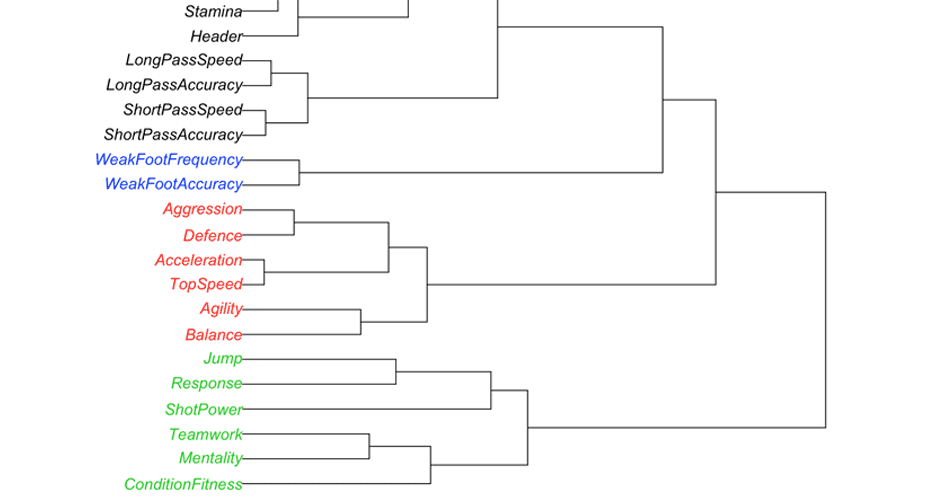
The next step, and probably the one we should have done first is Hierarchical Clustering. This can show us the tree or dendogram.
movementScreenData.HCWard <- hclust(d = dist(movementScreenData), method = "ward")

plot(movementScreenData.HCWard, xlab = "", ylab = "", yaxt = "n", main = "Ward Method")

rect.hclust(movementScreenData.HCWard, k = 4)
What we can see is that the buckets differ between the methods. This depends on the method selected. In the next picture we can see the hierarchical clustering result by using different method
movementScreenData.HCComplete <- hclust(d = dist(movementScreenData), method = "complete")

plot(movementScreenData.HCComplete, xlab = "", ylab = "", yaxt = "n", main = "Complete Method")

rect.hclust(movementScreenData.HCComplete, k = 4)
Here are the athletes list and the buckets based on different methods of clustering
athletes.buckets <- data.frame(Name = names(movementScreenData.K4$cluster),
    `K-Means Bucket` = movementScreenData.K4$cluster, `Ward Bucket` = cutree(movementScreenData.HCWard,
        k = 4), `Complete Bucket` = cutree(movementScreenData.HCComplete, k = 4))

# Remove the row names
row.names(athletes.buckets) <- NULL

# Print the table
print(xtable(athletes.buckets, digits = 2), type = "html")
| Name | K.Means.Bucket | Ward.Bucket | Complete.Bucket | |
|---|---|---|---|---|
| 1 | Vigil Sandoval, Ashley | 3 | 1 | 1 |
| 2 | Trumpore, Gabriela | 1 | 2 | 2 |
| 3 | Haddenham, Stephanie | 2 | 3 | 2 |
| 4 | Archuleta, Cameron | 1 | 4 | 3 |
| 5 | Oliva, Haile | 2 | 3 | 2 |
| 6 | Alfandi, Adan | 2 | 3 | 2 |
| 7 | Rodriguez, Morgan | 1 | 4 | 3 |
| 8 | Martinez, Kellie | 2 | 3 | 2 |
| 9 | Crowe, Aaron | 4 | 4 | 3 |
| 10 | Li, Isidro | 1 | 2 | 4 |
| 11 | Marquez, Ashley | 2 | 3 | 2 |
| 12 | Sanchez-Chavez, Daryl | 2 | 3 | 2 |
| 13 | Sauls, Anthony | 1 | 4 | 3 |
| 14 | Jordan, Michael | 3 | 1 | 1 |
| 15 | Cade, Christina | 4 | 4 | 3 |
| 16 | Han, Kenny | 2 | 3 | 2 |
| 17 | Sherer, Manuel | 1 | 4 | 3 |
| 18 | Black, Oswald | 2 | 1 | 2 |
| 19 | Vue, Marcus | 1 | 4 | 3 |
| 20 | Johnson, Laurencita | 2 | 2 | 4 |
| 21 | Klose, Alexander | 4 | 4 | 3 |
| 22 | Magill, Michaellee | 1 | 2 | 2 |
| 23 | Johnson, Santos | 2 | 1 | 2 |
| 24 | Martinez-Montenegro, Erasmo | 3 | 1 | 1 |
| 25 | Chamberlain, Samantha | 4 | 1 | 1 |
| 26 | Marin, Josiah | 2 | 3 | 2 |
| 27 | Gutierrez, Hunter | 3 | 1 | 1 |
Welcome to the real world 🙂 Again, the best approach might be to take into account number of factors and the gym conditioning and resources and use K-Means to perform clustering. Once I learn how to do PCA/EFA I will come back to this example again.
Did we miss something?
If we come back to the original data we loaded (movementScreenData), we can see that we have Age, Weight, Height, Body Fat, LBM, BMI, Limb.Length and Dominance collums. They are not Screening tests, so will we get different results if we kick them out? Let’s find out
# Remove first 8 columns
movementScreenData <- movementScreenData[, -1:-8]
Plot the K-Means clustering again
set.seed(10)

movementScreenData.K2 <- kmeans(x = movementScreenData, centers = 2)
movementScreenData.K3 <- kmeans(x = movementScreenData, centers = 3)
movementScreenData.K4 <- kmeans(x = movementScreenData, centers = 4)
movementScreenData.K5 <- kmeans(x = movementScreenData, centers = 5)

K2.Clusters <- plot(movementScreenData.K2, data = movementScreenData, title = "Two Clusters")
K3.Clusters <- plot(movementScreenData.K3, data = movementScreenData, title = "Three Clusters")
K4.Clusters <- plot(movementScreenData.K4, data = movementScreenData, title = "Four Clusters")
K5.Clusters <- plot(movementScreenData.K5, data = movementScreenData, title = "Five Clusters")

grid.arrange(K2.Clusters, K3.Clusters, K4.Clusters, K5.Clusters, ncol = 2)
It seems that now three clusters pretty much explain our results. Let’s plot the dendogram using Ward and Complete methods and create a list of athletes
# Ward
movementScreenData.HCWard <- hclust(d = dist(movementScreenData), method = "ward")

plot(movementScreenData.HCWard, xlab = "", ylab = "", yaxt = "n", main = "Ward Method")

rect.hclust(movementScreenData.HCWard, k = 3)
# Complete
movementScreenData.HCComplete <- hclust(d = dist(movementScreenData), method = "complete")

plot(movementScreenData.HCComplete, xlab = "", ylab = "", yaxt = "n", main = "Complete Method")

rect.hclust(movementScreenData.HCComplete, k = 3)
And create a list of athletes in buckets depending on the method
athletes.buckets <- data.frame(Name = names(movementScreenData.K3$cluster),
    `K-Means Bucket` = movementScreenData.K3$cluster, `Ward Bucket` = cutree(movementScreenData.HCWard,
        k = 3), `Complete Bucket` = cutree(movementScreenData.HCComplete, k = 3))

# Remove the row names
row.names(athletes.buckets) <- NULL

# Print the table
print(xtable(athletes.buckets, digits = 2), type = "html")
| Name | K.Means.Bucket | Ward.Bucket | Complete.Bucket | |
|---|---|---|---|---|
| 1 | Vigil Sandoval, Ashley | 3 | 1 | 1 |
| 2 | Trumpore, Gabriela | 3 | 2 | 2 |
| 3 | Haddenham, Stephanie | 3 | 1 | 1 |
| 4 | Archuleta, Cameron | 3 | 1 | 2 |
| 5 | Oliva, Haile | 3 | 1 | 1 |
| 6 | Alfandi, Adan | 3 | 1 | 1 |
| 7 | Rodriguez, Morgan | 3 | 1 | 1 |
| 8 | Martinez, Kellie | 2 | 1 | 1 |
| 9 | Crowe, Aaron | 2 | 3 | 1 |
| 10 | Li, Isidro | 2 | 3 | 2 |
| 11 | Marquez, Ashley | 3 | 1 | 1 |
| 12 | Sanchez-Chavez, Daryl | 1 | 1 | 1 |
| 13 | Sauls, Anthony | 3 | 1 | 1 |
| 14 | Jordan, Michael | 1 | 2 | 3 |
| 15 | Cade, Christina | 3 | 1 | 2 |
| 16 | Han, Kenny | 3 | 1 | 1 |
| 17 | Sherer, Manuel | 2 | 3 | 1 |
| 18 | Black, Oswald | 1 | 2 | 1 |
| 19 | Vue, Marcus | 2 | 3 | 1 |
| 20 | Johnson, Laurencita | 1 | 2 | 3 |
| 21 | Klose, Alexander | 2 | 3 | 1 |
| 22 | Magill, Michaellee | 3 | 2 | 2 |
| 23 | Johnson, Santos | 1 | 2 | 1 |
| 24 | Martinez-Montenegro, Erasmo | 3 | 1 | 2 |
| 25 | Chamberlain, Samantha | 2 | 2 | 2 |
| 26 | Marin, Josiah | 1 | 2 | 2 |
| 27 | Gutierrez, Hunter | 1 | 1 | 2 |
Summary
Here is the summary of what I’ve learned from the above examples when performing Cluster Analysis
- Make sure you use the right data. The Data Analysts use ~80% of their time to prepare the data – they call it data munging. It is dirty, but most important (see the differences above when we excluded some data)
- As with fitness testing, results are protocol dependent. Make sure to know the pros and cons of each
- Use common sense and real life constraints (how many groups you can serve?)
- Know underlying qualities/factors (perform PCA/EFA) – how many different factors are involved in the data set (e.g. mobility, stability)
- Try to see what factors/qualities each athlete bucket are missing.
The number 5 is my next step in this type of analysis. The goal is to make life of the coaches easier in the end.
The Cluster analysis can be performed on various types of data, like game performance data (to see how the positions differ and if), player profiles (again optimizing approach for different groups). I will write more about it as I learn more about it 🙂
If I made any error here please let me know. I have created a thread on the forum for further questions/ideas





Responses