Decoding Fatigue: Can We Measure It Live in Team Sports? – Part 2
Introduction
In the previous installment, we explored the complexity of fatigue. Now, we need to take a step forward—not by making it less complex, but by operationalizing it.
Defining Performance Limits: A Thought Experiment
Imagine you’re performing a bench press with 100 kg for five reps, pushing to absolute failure (zero reps in reserve, or RIR = 0). Are you tired afterward? Absolutely. But if we measured your maximal isometric force immediately after, would it be lower than before?
I can’t say for certain, as I’m not aware of a study examining this exact scenario (if you know of one, let me know). However, based on research like Marcora’s work on fatigue perception (Marcora and Staiano 2010), I would speculate that while maximal force output may decrease, it wouldn’t drop below 100 kg.
This highlights an important point: we can theorize about fatigue mechanisms indefinitely, but at the end of the day, what truly matters is whether an athlete reaches their performance limit. That limit is context-dependent—meaning motivation, pressure, music, or competition could all push an athlete to perform more reps. So if the same athlete does fewer reps on another day, is it due to fatigue or simply normal fluctuation? That’s difficult to determine, but knowing an athlete’s performance ceiling provides a reference point to interpret changes.
Applying This to Running
Since we’re focused on running-based team sports, let’s translate this concept to running.
Suppose an athlete’s performance limit for a 1,500m run is 3:20. If they intentionally run at a submaximal pace, their fatigue will likely be lower. But here’s the question: if they complete the distance 20% slower than their max effort, does that mean they are experiencing 20% less fatigue?
I don’t have a definitive answer, but this proximity to performance limits could serve as a valuable insight—one that aligns with Andrea Zignoli’s Workout Reserve Model (Zignoli 2023), which I’ll discuss later.
Expanding to Multiple Distances
What if we know an athlete’s 1,500m performance limit but want to predict their 3,000m limit? This is similar to testing a bench press max at 100 kg, 120 kg, and 80 kg. Experience tells us that as the distance increases, average running velocity decreases—just like adding weight to the bar reduces the number of reps possible.
These are robust phenomena of the Large World—patterns that emerge consistently in real-world performance. But to describe, predict, and intervene, we need to create models—our Small Worlds—that simplify and map these patterns mathematically.
In this article series, I’ll introduce one such model, but keep in mind that there are multiple Small World models that can be applied, each offering unique insights.
Table 1 enlists performance results across different distances, while Figure 1 presents them graphically.
| Distance [m] | Time [m:s] | Velocity [km/h] |
|---|---|---|
| 1500 | 6:26 | 14.0 |
| 2000 | 8:49 | 13.6 |
| 4000 | 18:20 | 13.1 |
| 6000 | 27:51 | 12.9 |
Table 1: Performance over different distances
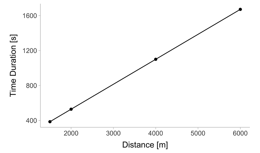
(a) Time versus Distance
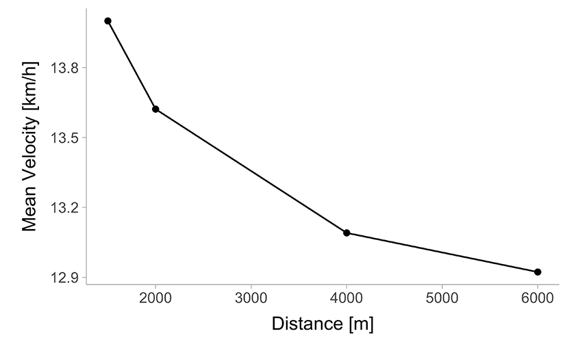
(b) Mean Velocity versus Distance
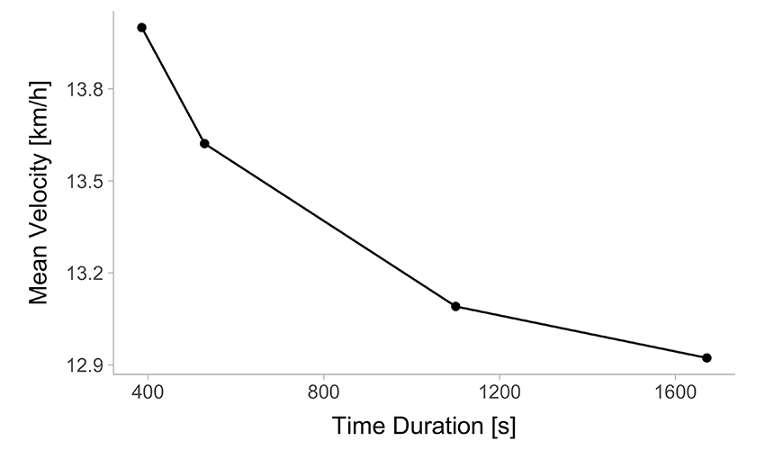
(c) Mean Velocity versus Time Duration
Figure 1: Graphical representation of the Table 1
We want to map out these relationships (Figure 1) using a specific Small World model whose parameters have physiological significance. This can help us extract certain latent qualities—or perhaps more accurately, compress them—depending on whether we assume a formative or reflective model.
Either way, Small World models provide a structured way to navigate performance data, helping us estimate time trial performance at distances that were not directly measured. Of course, multiple modeling approaches (Small Worlds) can be used to achieve this.
A simple linear regression (Figure 2 (a)) assumes a direct proportionality, but we can immediately see that this assumption is flawed. A polynomial model fit (Figure 2 (b)) offers a better representation of the data, yet it comes with its own problems—such as unreliable extrapolation beyond the observed range and a lack of physiological interpretability in its estimated parameters.
To truly make this approach useful, we need a model that not only fits the data well but also aligns with physiological principles.
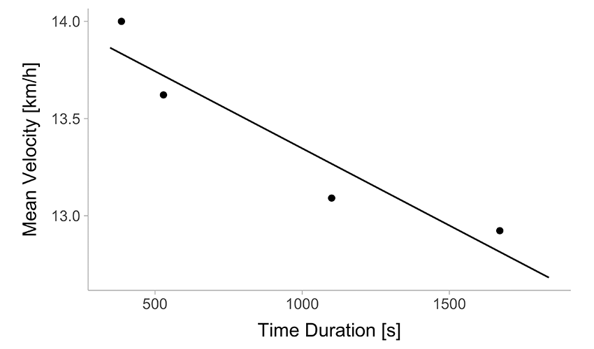
(a) Simple linear regression
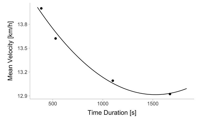
(b) Polynomial linear regression
Figure 2: Simple regression models of the velocity~duration
Critical Velocity Model
One of the most popular models for mapping mean velocity against time duration is the Critical Velocity (CV) model (Equation 1).
\[
v(t_{lim}) = \frac{D'}{t_{lim}} + CV
\tag{1}\]
The Critical Velocity (CV) model has two key parameters:
- Critical Velocity (CV) – the velocity that, in theory, one can sustain indefinitely. It is closely related to the anaerobic threshold or the second ventilatory threshold, though it may be slightly higher.
- \(D'\) (D prime) – representing anaerobic capacity, which acts as a finite energy buffer. Every time an athlete runs faster than CV, this buffer is depleted, with the rate of depletion depending on how much the velocity exceeds CV—i.e., the faster you run, the quicker you exhaust \(D'\).
This model is both simple and elegant, as its parameters align well with our a priori understanding of physiology.
Using non-linear regression, we can estimate the model parameters from Equation 1, resulting in:


Nice work on this Mladen, I have a student working in a similar space. Any chance you have or would be able to make the D’balance code for the above analysis available? There is also a paper by Mizelman et al. (2024) where they explore this and introduce an R package to apply to GPS/GNSS datasets.
Hi Mitch, glad you like the series. Can you shoot me your email in PM here on site and I will send you the code