Sprint Variability Profiling: New Insights From Speed Testing Data
The old adage in team sports is that “speed kills” but what if faulty interpretation of speed testing data is killing our ability to meaningfully assess and assist our athlete’s sprint performance?
The typical approach for speed assessment of team sport athletes is to test athletes over a 40 m distance with their “output” tracked at various 10 m intervals in between – giving the coach 10 m, 20 m, 30 m and/or 40 m sprint times. Often in the team sport environment we look at 10 m time as a global indicator of acceleration with our total 40 m times highlighting top speed characteristics. ‘’We typically use rankings to benchmark players against each other or against “normative” data we have accrued over time. Ranking lists are shared and promoted to praise the best accelerators or our top speed kings.
But rankings are deceptive and offer very little practical insight into our athletes’ true speed qualities. They do not tell us the real difference between players. Only a hundredth of a second may separate an athlete ranked 1st to 2nd on a ranking list – well within true meaningful difference. Yet a tenth of a second might separate 2nd to 3rd. Rankings are ordinal variables and tell us nothing of the magnitude of difference. However, on a ranking list hung in the gym or the locker-room 1st to 2nd is enough for bragging rights regardless of the true difference.
While outcome is important (“who is the fastest over 40 m?”) as coaches we should be more interested in what contributes to that outcome and where opportunities for performance enhancement lie. For us, it is not just “what you do” but “how you do it”. If we understand the “how”, then we can be one step closer to crafting performance enhancement strategies.
The holy grail for coaches and sport scientists is to derive additional insight and competitive advantage from existing protocols and datasets – without any additional data collection. We aim to offer such a solution for speed testing data in this article.
A common mistake made by S&C coaches, with respect to speed testing data is that a 40 m time is assumed to be representative of top speed ability. However, a total 40 m time is an all-encompassing “outcome” variable and contained within it is 0-10 m times much more representative of accelerative ability. So for example, an athlete with exceptional short-acceleration ability over 10 m may be distinctly average from 30-40 m but he has already put enough distance between him and the opposition to finish with a top ranking 40 m time. So we assume “good top speed” but the reality is “top accelerator, average-to-poor top speed”. From our anecdotal experience, the reverse is even more common. Some athletes have poor acceleration but relatively higher maximum velocity abilities – a combination which yields merely an “average” 40m time1. Martin Bucheit, head of performance at Paris St. Germain football club, has empirically demonstrated examples of these “profile-types” in his 2014 paper “Mechanical determinants of acceleration and maximal sprinting speed in highly trained young soccer players”1.
Splits on the other hand isolate out a particular phase of sprint performance. A split time from 30-40 m is much more specifically representative of what is happening in the top speed phase. By examining outcomes (10 m, 20 m, 30 m, 40 m times) and splits (10 m, 10-20 m, 20-30 m, 30-40 m) together we get a better picture of “what we do” and “how we do it”. While track athletes have combined splits and outcomes in their training practice for eternity, the practice is much less common in field sport athletes where outcome scores like the 10 m and 40 m total time tend to be lionised. In field sports, benchmarking data is not generally used for split times. Coaches have a strong sense of what constitutes good or bad 10 and 40 m times – outcome is generally at the forefront of a coach’s mind. However, we don’t typically have as robust an understanding of how good or bad specific split times are.
What we really want is a ranking based system but which also takes into account the magnitude of differences between athletes AND allows us to derive insight into the different phases of early acceleration, late acceleration and top-speed running. We need an analysis tool which considers both outcomes and splits and allows us to identify gaps in performance.
Sprint variability profiling, using statistical z-scores can be this tool.
The z-score is a standardised score which tells us how many standard deviations you are better, or worse, than the average of your group. In a z-scoring system, the mean data is represented as a 0 value. If an athlete’s 10 m time is the exact same as the group average, then that athlete’s score presents as a 0. An athlete with a z-score of 1 would be 1 standard deviation above the mean data point for a particular variable. A z-score of -1 would be 1 standard deviation below average.
A sprint variability profiling system allows us the opportunity to combine outcomes and splits in our analyses and highlights athletes’ performance strengths and weaknesses relative to the variability within their group of peers. It tells us how good each athlete is overall but also in each section of sprint performance relative to the group. It’s a visual, intuitive tool that allows us to see the “what” and the “how”.
We start the process by pooling together all our group data, finding a group mean and assessing the group variance by calculating a standard deviation for each outcome (10 m, 20 m, 30 m & 40 m time) and for each split (0-10 m, 10-20 m, 20-30 m, 30-40 m split times). We use athletes’ fastest sprint from speed testing so that each split is “connected” and the outcomes are the direct result of cumulative splits.
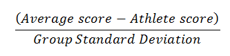
Figure 1 shows the z-scores for a field sport athlete for his “outcome” measures only. Each outcome time (10, 20, 30, 40 m) is converted to a z-score relative to this player’s “group” using the equation:
The representative group could be the player’s squad or a large group of players of similar position. The coach must be aware that the group will affect our insight on what the “rate-limiters” are for individual athlete. The technique lives or dies based on the quality of the normative dataset. Ideally groups will be as specific as possible for maximum validity. For example, in a sport like rugby union, players should be split into backs and forwards groups at the very least, but further refinement to create position specific norms would offer even greater relevance of insight. A good rule of thumb would be to match athletes based on general speed qualities that are desirable for their position. Coaches must also remember that normative data must have a critical mass of sample size to be valid. If possible, we recommend normative reference groups of approximately 15-20 athletes of similar positional demands.
A quick technical note: In the context of sprint times we “flip” the traditional z-score formula. A better speed time is faster and thus lower than the average represented by a negative z-score. However, we prefer to flip the calculation so that graphs and charts are more intuitive and the best performers are highest on the chart and an above average speed qualities are represented by positive z-scores. See example chart below.
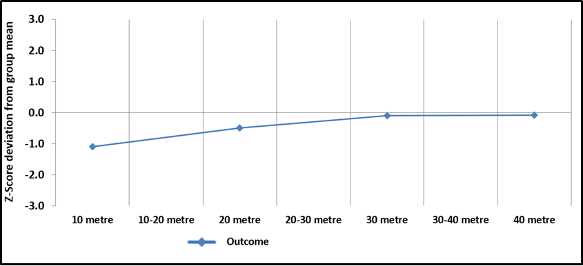
The outcome data for the athlete in figure 1 has a clear “positive profile”. A poor 10 m time which is one standard deviation below average but increasing performance across the duration of the sprint means he finishes with an “average” 40 m outcome. A limited interpretation here would suggest the athlete has poor acceleration skills but rescues performance with better top speed running. When we overlay our split data, again converted to z-scores relative to the group, then we get a little more insightful detail.
Co-Author
Robin Healy is a sports biomechanics Ph.D. candidate at the Biomechanics Research Unit of the University of Limerick (UL) where he works primarily with sprint athletes. He has previously consulted with the Sport Ireland Institute and was a former intern S&C coach with Munster Rugby. Robin is available for collaboration on sprint variability profiling and data analysis projects with coaches, teams and athletes.


Responses