Sprint Profiling – Common Problems and Solutions Part 2
Previous Part:
 Sprint Profiling – Common Problems and Solutions Part 1
Tether device or the analysis of the distance-velocity trace
In the previous part, we have discussed the analysis of the time-velocity trace provided by the radar or laser gun. But if you remember, I have actually used the DynaSpeed(TM) dataset (using data("dynaspeed")). DynaSpeed(TM) is a tether device (Figure 1) that besides providing measurement can also provide resistance or assistance. It is indeed outstanding piece of technology. The resisted aspects of sprinting, and modeling of the same, will be dealt in the upcoming article. For now, we will deal with the measurement aspects.
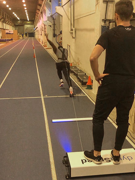
Figure 1: Sprinting with DynaSpeed(TM). Image courtesy of Håkan Andersson
DynaSpeed(TM) provides time, distance, and velocity metrics (as well as forces and accelerations and many others). In the previous installment of this article series we have created sprint profile using the time-velocity trace. In this section we will wrestle with the distance-velocity trace (Figure 2).
Show/Hide Code
library(tidyverse)
library(shorts)

data("dynaspeed")

gg <- dynaspeed %>%
  ggplot(aes(x = distance)) +
  geom_line(aes(y = raw_velocity), alpha = 0.3, linewidth = 0.25) +
  geom_line(aes(y = velocity), alpha = 0.9, linewidth = 0.5) +
  ylab("Velocity (m/s)") +
  xlab("Distance (m)") +
  scale_x_continuous(expand = c(0, 0), limits = c(0, NA)) +
  scale_y_continuous(expand = c(0, 0), limits = c(0, NA))

gg
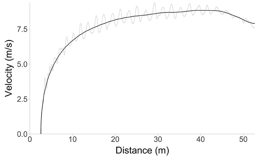
Figure 2: Sample data from DynaSpeed(TM) from data("dynaspeed") dataset in {shorts} package
As opposed to the time-velocity trace, the distance doesn’t flow if the athlete stands still when the measurement begins. Figure 2 represents the same sprint we have analysed in the previous installment using the time-velocity trace.
The DynaSpeed(TM) dataset (i.e., data("dynspeed")) which comes with the {shorts} package involves intentional time and distance shifts cause by yours truly. This is done to provide analysis sandbox for this article series, and it doesn’t represent a flaw in the DynaSpeed(TM) system.
But how do we define the mono-exponential model for the distance-velocity trace? We have already introduced Equation 1, but how do we modify it to predict velocity at distance?
\[
v(t) = MSS \cdot \left(1 – e^{-\frac{t}{TAU}}\right)
\tag{1}\]
To do so, we can take the route of predicting time at distance, but we have only introduced Equation 2, which predicts distance at time (i.e., it has the predictor and outcome flipped).
\[
d(t) = MSS \cdot \left(t + TAU \cdot e^{-\frac{t}{TAU}}\right) – MSS \cdot TAU
\tag{2}\]
With a little bit of help by Wolfram Alpha (or OpenAI ChatGPT), particularly for those who suck at math like myself, we can solve the Equation 2 for predicting time at distance. The solution is shown in Equation 3 and it involves Lambert W function (it is beyond my knowledge and motivation to explain it here).
\[
t(d) = TAU \cdot W\left(-e^{\frac{-d}{MSS \cdot TAU}} – 1\right) + \frac{d}{MSS} + TAU
\tag{3}\]
We will be actually using Equation 3 when dealing with timing-gates/photocells, but more about it in the next installment. Anyway, now we can predict the time at distance. So we can chug Equation 3 into Equation 1 (i.e., Equation 4) to get equation for predicting velocity at distance.
\[
v(d) = v(t(d))
\tag{4}\]
The result of our efforts can be found in Equation 5.
\[
v(d) = MSS \cdot \left(1 – e^{-\left(\frac{TAU \cdot W\left(-e^{-\frac{d}{MSS \cdot TAU}} – 1\right) + \frac{d}{MSS} + TAU}{TAU}\right)}\right)
\tag{5}\]
This model definition is implemented in the model_tether() function in the {shorts} package. But due to issues in measurement (i.e., inability of the athlete and device to start the sprint/measurement at exactly \(d=0m\)), we do need to implement certain type of correction or intercept, similarly to what we have done with time-velocity trace in previous installment.
This correction, titled distance correction (DC) can easily be added to Equation 5 by subtracting \(DC\) from distance. Please refer to Equation 6 for a solution. This model definition is implemented in the model_tether_DC() function in the {shorts} package. Although I tried to implement the \(DC\) parameter automatically to the model_tether() function, like I have done with the \(TC\) in the model_laser() function, I had issues in model fitting when there is no distance shift in the data (sorted out by filtering \(velocity > 0\)). Thus I have provided an option for the user – maybe in the future versions of the {shorts} package I will opt for only one tether function which has \(DC\) automatically.
\[
v(d) = MSS \cdot \left(1 – e^{-\left(\frac{TAU \cdot W\left(-e^{-\frac{d – DC}{MSS \cdot TAU}} – 1\right) + \frac{d – DC}{MSS} + TAU}{TAU}\right)}\right)
\tag{6}\]
Now that we have the model definition, let’s train the model using the data from Figure 2. Similarly to time-velocity trace, we do need to filter out only the short sprint by removing the deceleration at the end. Since the distance is not changing when athlete is standing, we do not need to deal with that issue with the distance-velocity trace. But the other problem might emerge, and that is the negative velocity, particularly if we are using the raw velocity, which can happen due to body sway when standing still, or having zero velocity which did affect model fitting in my experience (not sure why though – this is some math stuff, which is beyond my comprehension). It is thus recommended that we also filter out minimal velocities, e.g., everything below 0.1 \(ms^{-1}\). To achieve this we will again use the smoothed velocity provided by the system.


Responses