R Playbook: Introduction to Mixed-Models

I just started reading more about mixed-models (multilevel/hierarchical) and will use this as a playbook. Mostly becaus I learn the best by experimenting with the data and I suggest everyone to try to do the same. So please note that this is just a published playbook – if you find it useful, great, if you find some errors, please let me know, if you find it useless, well, disregard it.

Anyway, here is our sleep study data from lme4 package:

The data represents the average reaction time per day for subjects in a sleep deprivation study. On day 0 the subjects had their normal amount of sleep. Starting that night they were restricted to 3 hours of sleep per night. The observations represent the average reaction time on a series of tests given each day to each subject.
Basically repeated measures design. Let’s see the relationship between days and reaction time.

gg <- ggplot(sleepstudy, aes(x = Days, y = Reaction))
gg <- gg + geom_point(color = "blue", alpha = 0.7)
gg <- gg + geom_smooth(method = "lm", color = "black")
gg <- gg + theme_bw()
gg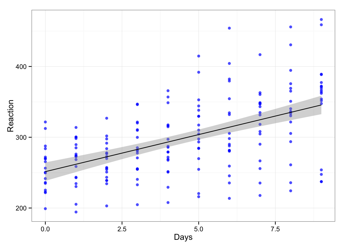

If we create simple linear model we get the following

model1 <- lm(Reaction ~ Days, sleepstudy)
summary(model1)

## 
## Call:
## lm(formula = Reaction ~ Days, data = sleepstudy)
## 
## Residuals:
##      Min       1Q   Median       3Q      Max 
## -110.848  -27.483    1.546   26.142  139.953 
## 
## Coefficients:
##             Estimate Std. Error t value Pr(>|t|)    
## (Intercept)  251.405      6.610  38.033  < 2e-16 ***
## Days          10.467      1.238   8.454 9.89e-15 ***
## ---
## Signif. codes:  0 '***' 0.001 '**' 0.01 '*' 0.05 '.' 0.1 ' ' 1
## 
## Residual standard error: 47.71 on 178 degrees of freedom
## Multiple R-squared:  0.2865, Adjusted R-squared:  0.2825 
## F-statistic: 71.46 on 1 and 178 DF,  p-value: 9.894e-15

And our coefficients are the following:

coef(model1)

## (Intercept)        Days 
##   251.40510    10.46729

What we learned from the model is that days with sleep deprivations are negativelly affecting reaction time. The 95% CIs are:

round(confint(model1), 2)

##              2.5 % 97.5 %
## (Intercept) 238.36 264.45
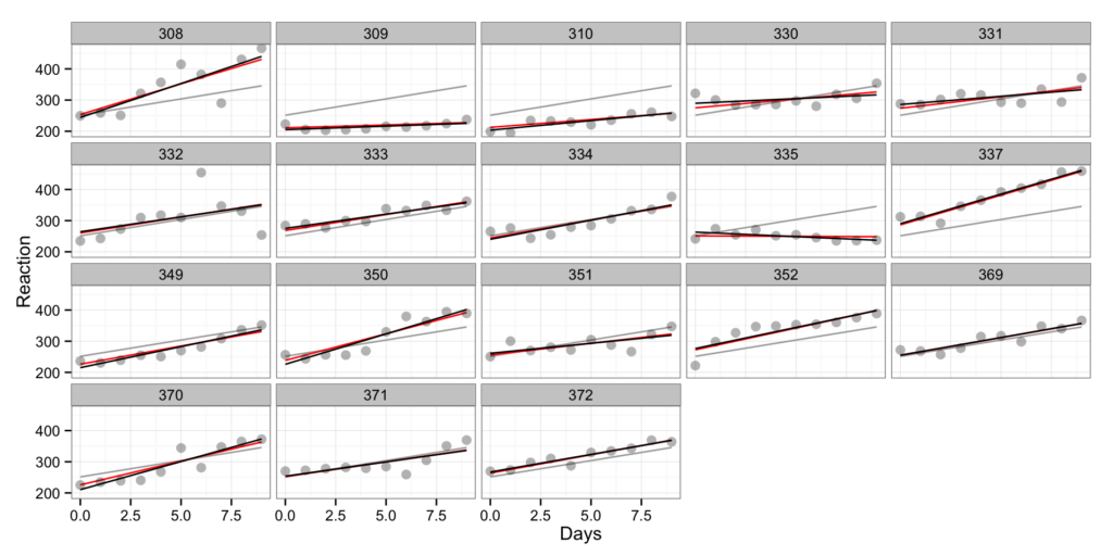
## Days          8.02  12.91

But we included all the subjects into one bin and there is probably variation within the subjects. Let’s plot the trellis graph across the subjects:

gg <- gg + facet_wrap(~Subject)
gg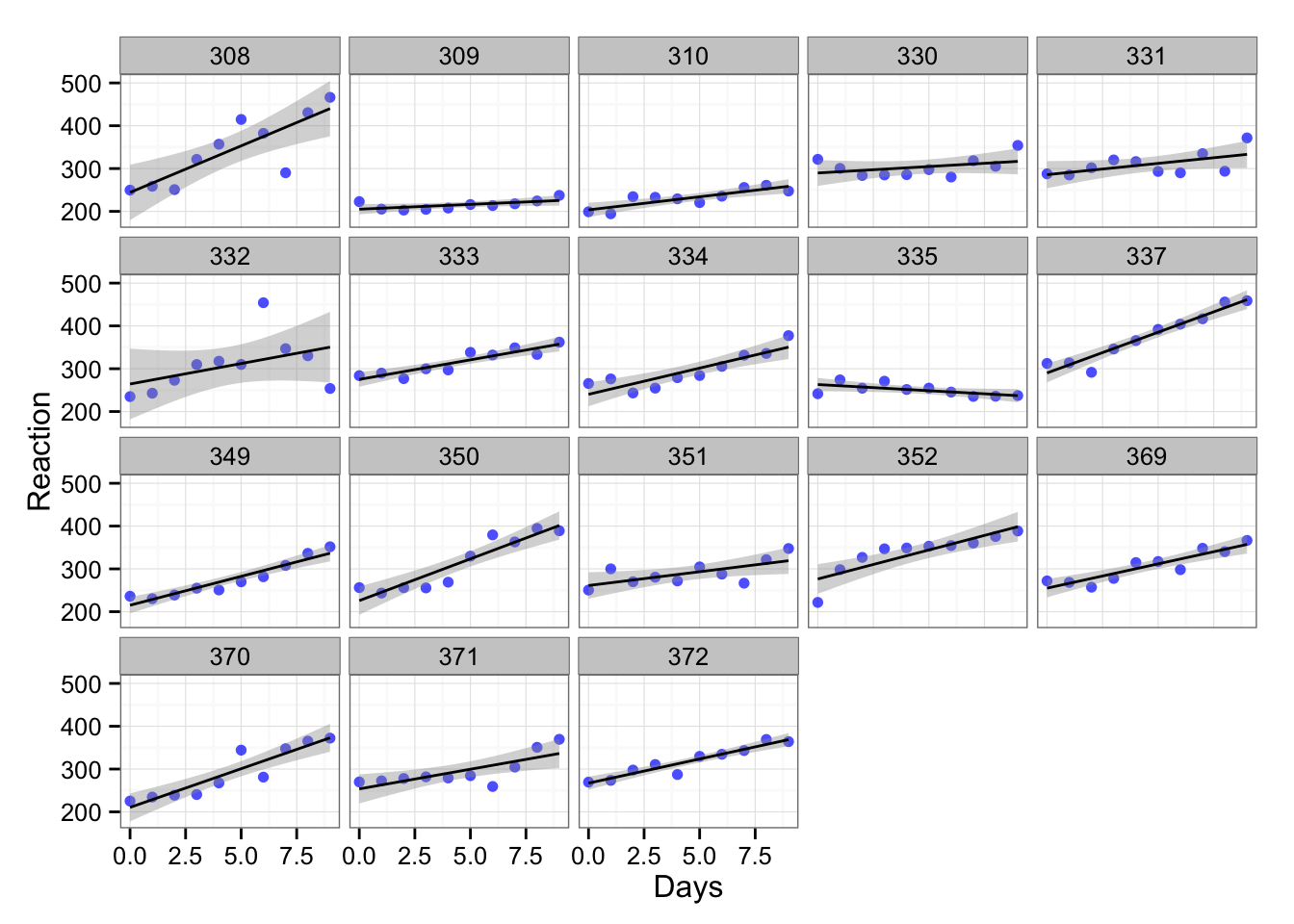

In the above graph each subject is depicted in single box (the number above is the code of the subject). As we can see the subject reaction differs. What we can do is to create linear model for each subject. Let’s do it for subject 308 and subject 335

model308 <- lm(Reaction ~ Days,
               data = subset(sleepstudy, Subject == 308))
model335 <- lm(Reaction ~ Days,
               data = subset(sleepstudy, Subject == 335))

summary(model308)

## 
## Call:
## lm(formula = Reaction ~ Days, data = subset(sleepstudy, Subject == 
##     308))
## 
## Residuals:
##      Min       1Q   Median       3Q      Max 
## -106.397   -4.098    9.688   22.269   61.674 
## 
## Coefficients:
##             Estimate Std. Error t value Pr(>|t|)    
## (Intercept)   244.19      28.08   8.695 2.39e-05 ***
## Days           21.77       5.26   4.137  0.00326 ** 
## ---
## Signif. codes:  0 '***' 0.001 '**' 0.01 '*' 0.05 '.' 0.1 ' ' 1
## 
## Residual standard error: 47.78 on 8 degrees of freedom
## Multiple R-squared:  0.6815, Adjusted R-squared:  0.6417 
## F-statistic: 17.12 on 1 and 8 DF,  p-value: 0.003265

summary(model335)

## 
## Call:
## lm(formula = Reaction ~ Days, data = subset(sleepstudy, Subject == 
##     335))
## 
## Residuals:
##      Min       1Q   Median       3Q      Max 
## -21.4264  -3.8697  -0.1774   4.5403  16.4105 
## 
## Coefficients:
##             Estimate Std. Error t value Pr(>|t|)    
## (Intercept)  263.035      6.694  39.296 1.93e-10 ***
## Days          -2.881      1.254  -2.298   0.0506 .  
## ---
## Signif. codes:  0 '***' 0.001 '**' 0.01 '*' 0.05 '.' 0.1 ' ' 1
## 
## Residual standard error: 11.39 on 8 degrees of freedom
## Multiple R-squared:  0.3976, Adjusted R-squared:  0.3223 
## F-statistic:  5.28 on 1 and 8 DF,  p-value: 0.05065

Subject 308 have positive coefficient (and statistically significant), where subject 335 have negative coefficeint (and nearly statistically significant).

round(confint(model308), 2)

##              2.5 % 97.5 %
## (Intercept) 179.43 308.95
## Days          9.63  33.90

round(confint(model335), 2)

##              2.5 % 97.5 %
## (Intercept) 247.60 278.47
## Days         -5.77   0.01

Let’a create linear models across subjects

model2 <- lmList(Reaction ~ Days | Subject, sleepstudy)
model2.coefficients <- coef(model2)
names(model2.coefficients) <- c("Intercept", "Days.Slope")

We have intercept and slope for each subject
And we can plot them:

gg <- ggplot(model2.coefficients, aes(x = Intercept, y = Days.Slope))
gg <- gg + geom_point()
gg <- gg + theme_bw()
gg <- gg + geom_smooth(method = "loess")
gg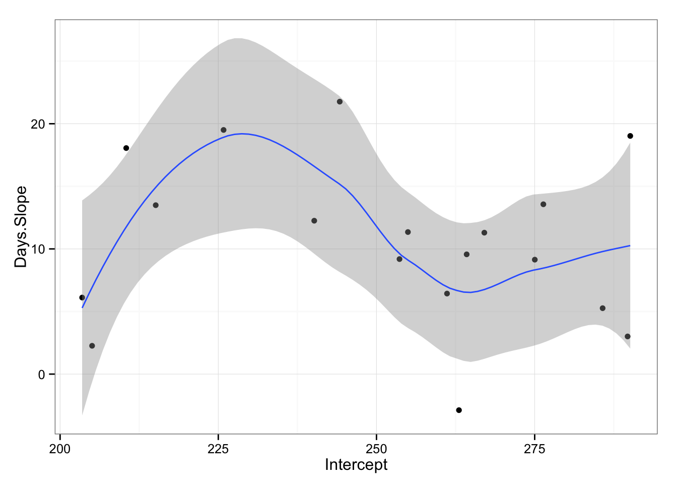

What we are interested to see from the graph is that if there is relationship from starting reaction time and slope across subjects. As can be seen from the picture it appears that there is non-linear relationship. We can also try to apply linear model (even if we can see that things are not linear) just to check for the trend.

gg <- ggplot(model2.coefficients, aes(x = Intercept, y = Days.Slope))
gg <- gg + geom_point()
gg <- gg + theme_bw()
gg <- gg + geom_smooth(method = "lm")
gg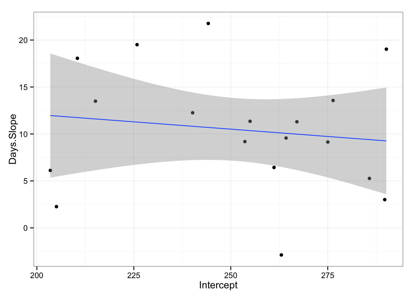

model3 <- lm(Days.Slope ~ Intercept, model2.coefficients)
summary(model3)

## 
## Call:
## lm(formula = Days.Slope ~ Intercept, data = model2.coefficients)
## 
## Residuals:
##      Min       1Q   Median       3Q      Max 
## -12.9860  -4.0312   0.2458   3.3818  11.0727 
## 
## Coefficients:
##             Estimate Std. Error t value Pr(>|t|)
## (Intercept) 18.30016   14.18878   1.290    0.215
## Intercept   -0.03116    0.05609  -0.555    0.586
## 
## Residual standard error: 6.696 on 16 degrees of freedom
## Multiple R-squared:  0.01892,    Adjusted R-squared:  -0.0424 
## F-statistic: 0.3086 on 1 and 16 DF,  p-value: 0.5862

As can be seen the trend is that subjects with slower initial reaction time have slower slope (or decrement) on their reaction time with sleep deprivation (not statistically significant, p = 0.582). Hence, slower individuals are less affected by sleep deprivation, even if the fixed effect is that everyone is affected by sleep deprivation negativelly (increase in reaction time, p < 0.001 ).
This can be easily performed using lme4 package.

mix.model1 <- lmer(Reaction ~ Days + (Days | Subject), sleepstudy)
summary(mix.model1)

## Linear mixed model fit by REML ['lmerMod']
## Formula: Reaction ~ Days + (Days | Subject)
##    Data: sleepstudy
## 
## REML criterion at convergence: 1743.6
## 
## Scaled residuals: 
##     Min      1Q  Median      3Q     Max 
## -3.9536 -0.4634  0.0231  0.4634  5.1793 
## 
## Random effects:
##  Groups   Name        Variance Std.Dev. Corr
##  Subject  (Intercept) 612.09   24.740       
##           Days         35.07    5.922   0.07
##  Residual             654.94   25.592       
## Number of obs: 180, groups:  Subject, 18
## 
## Fixed effects:
##             Estimate Std. Error t value
## (Intercept)  251.405      6.825   36.84
## Days          10.467      1.546    6.77
## 
## Correlation of Fixed Effects:
##      (Intr)
## Days -0.138

To be honest, I can understand a little bit of the lme4 model output. Anyway, we managed to take into acount the levels (in this case individual athletes) can create a model that calculates overal effects (fixed effects) of days of sleep deprivation to reaction time, but also take into account invidual differences and effect of starting reaction time (intervcept) to the slope (or effect of sleep deprivation) for each individual.

Back to the bat cave. To be continued…..

In the mean time I am reading the following book: