Optimal Force-Velocity Profile for Sprinting: Is It All Bollocks? – Part 6
In this sixth and final installment of this article series, I will explore whether the “causal” interpretation of the Force-Velocity Profiling (FVP; $F_0$, $V_0$ or their other combination variant $P_{max}$ and $S_{fv}$) “holds water” using N=1 testing. Ideally, this should be done with more athlete, which we might actually do in the near future, but for now a simple common sense and one athlete sprinting is more than enough to simulate the debate as well as to question FVP parameters as determinants of performance. You can read my initial beef with this model on Twitter here and here.
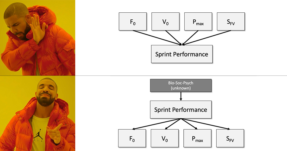
Purpose of the FVP (from the realist perspective) is to uncover mechanical determinants of sprinting, and further to consider them as causal traits of the individual responsible for sprint performance (Figure 1).
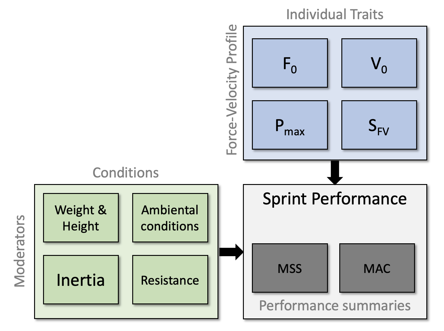
Figure 1: Realist viewpoint of assuming $F_0$ and $V_0$ to be causal determinants of performance and represent individual traits/qualities
This realist viewpoint sees FVP ($F_0$, $V_0$ and particularly their other combination variant $P_{max}$ and $S_{fv}$) as causal, responsible for sprint performance given the environmental conditions and constraints (e.g., wind speed and temperature, additional load or resistance and so forth).
We have already explored sensitivity of this model to changes in athlete body weight in terms of its effect of sprint performance (summarized by MSS and MAC parameters), assuming $F_0$ and $V_0$ stay the same. Here we will expand this theoretical model simulation by estimating changes in sprint performance under different types of environmental conditions.
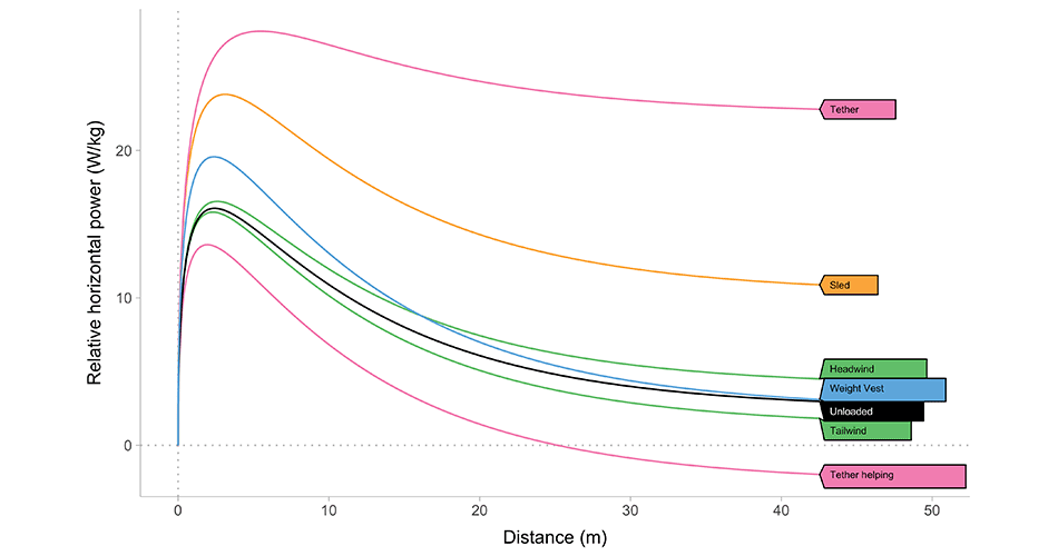
These conditions involve (1) extra horizontal resistance, in Newtons (force), but for the sake of simplicity expressed as kilograms (i.e., $100\;N = \frac{100}{9.81} = 10.19\;kg$), (2) additional inertia in a form of a weight vest, which only have vertical resistance but increase the athlete mass, and (3) a sled which is a combination of the two: providing extra inertia and horizontal resistance. For a sled, horizontal resistance (i.e., force) is assumed to be constant and equal to 0.4 of the sled weight (e.g., if the sled weights 20kg, then the horizontal resistance is equal to $20 \times 9.81 \times 0.4 = 78.5 \; N$).
If we assume that the $F_0$ and $V_0$, which are estimated during the normal sprinting, stay the same across conditions (and according to the realist model from Figure 1 they should since they represent individual traits or mechanical determinants), then we can estimate the sprint performance parameters changes. Here we assume we have athlete that weights 85 kg, height of 185 cm, with MSS and MAC equal to 9 $m^{-1}$ and 9 $m^{-2}$ respectively. Estimated $F_0$ and $V_0$ during normal sprint are equal to 680 N and 9.34 $m^{-1}$ respectively. These are considered to be mechanical determinants of this individual.
Then we increase the load used for resistance, vest, and sled conditions, from 0 to 25kg and estimate sprint performance parameters. Since I am bad at math, I will use optimization to do so.
Results are shown in Figure 2.
Show/Hide Code
# Generate data
require(tidyverse)
require(shorts)
require(kableExtra)
require(directlabels)

# ====================================
# Functions

# Total force
F_total <- function(MSS, MAC, BW, BH, inertia = 0, resistance = 0, velocity, ...) {
  slope <- MAC/MSS

  F_air <- get_air_resistance(velocity, bodymass = BW, bodyheight = BH, ...)
  F_acc <- (MAC - velocity * slope) * (BW + inertia)

  # Return total
  F_acc + F_air + resistance
}

# Make FV profile
find_FV <- function(MSS, MAC, BW, BH, inertia = 0, resistance = 0, ...) {

  F0 = F_total(MSS, MAC, BW, BH, inertia, resistance, velocity = 0, ...)

  find_V0 <- function(x) {
   F_total(MSS = MSS, MAC = MAC, BW = BW, BH = BH, inertia = inertia, resistance = resistance, velocity = x, ...)
  }

  V0 <- uniroot(find_V0, interval = c(0.01, 12), extendInt = "yes", tol = 10^-10)$root

  data.frame(F0 = F0, V0 = V0)
}

# Convert FV to AVP
find_AVP <- function(F0, V0, BW = 75, BH = 1.75, inertia = 0, resistance = 0, ...) {
  MAC <- (F0 - resistance) / (BW + inertia)
  find_V0 <- function(MSS) {
     V0 - find_FV(MSS, MAC, BW, BH, inertia, resistance, ...)$V0
  }

  MSS <- uniroot(find_V0, interval = c(0.01, 12), extendInt = "yes", tol = 10^-10)$root

  data.frame(
    MSS = MSS,
    MAC = MAC
  )
}

MSS <- 9
MAC <- 9
BW <- 85
BH <- 1.85
load <- 25

fvp <- find_FV(MSS, MAC, BW, BH, inertia = 0, resistance = 0)

# ====================================
# Simulation

# using friction coefficient, 0.4

# sensitivity
model_sens_df <- data.frame(
  init_MSS = MSS,
  init_MAC = MAC,
  F0 = fvp$F0,
  V0 = fvp$V0,
  BW = BW,
  BH = BH
) %>%
  expand_grid(
    load_type = c("vest", "resistance", "sled"),
    increment = seq(0, 1, length.out = 10)
  ) %>%
  rowwise() %>%
  mutate(
    new_inertia = ifelse(load_type == "resistance", 0, load * increment),
    new_resistance = ifelse(
      load_type == "vest", 0,
      ifelse(load_type == "resistance", 9.81 * load * increment, 9.81 * load * increment * 0.4))
  ) %>%
  mutate(data.frame(find_AVP(F0, V0, BW, BH, new_inertia, new_resistance))) %>%
  mutate(
    MSS = 100 * (MSS - init_MSS) / init_MSS,
    MAC = 100 * (MAC - init_MAC) / init_MAC) %>%
  pivot_longer(cols = c(MSS, MAC), names_to = "param")

ggplot(model_sens_df, aes(x = increment * load, y = value, color = param)) +
  theme_linedraw(8) +
  geom_line(alpha = 0.8) +
  geom_dl(
    aes(label = paste("  ", param)),
    method = list("last.bumpup", cex = 0.5)
  ) +
  ylab("Parameter Change (%)") +
  xlab("Load (kg)") +
  theme(legend.position = "none") +
  facet_wrap(~load_type, scales = "free_x") +
  xlim(0, 30)
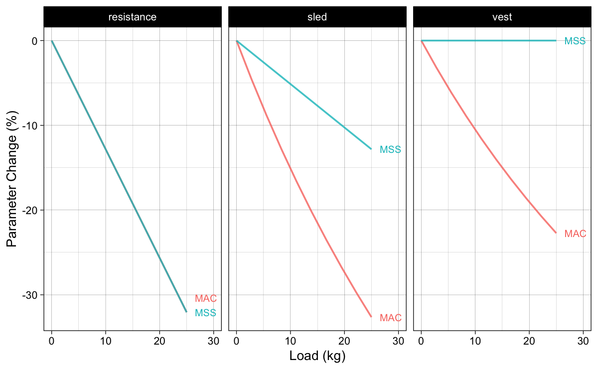
Figure 2: Assuming $F_0$ and $V_0$ are causal mechanical determinants (i.e., unchangable traits), we can estimate sprint performance (i.e., MSS and MAC) under different conditions. Resistance represents only horizontal resistance without inertia (i.e., force in Newtons, but here expressed in kg by dividing with 9.81 to align the scales). Sled represent pulling a sled, which is a combination of inertial load (i.e., mass in kg) and friction resistance, which is assumed to be 0.4 (e.g., pulling 10kg sled yield also $10 \times 9.81 \times 0.4 = 40\;N$). Vest represents only inertial load since there is no horizontal resistance/force
Assuming realist model of F_0 and V_0 being mechanical causal determinants or traits (Figure 1), results from Figure 2 indicate that changing external horizontal resistance (most likely provided using tether devices like Dynaspeed) negatively affect the sprint performance by decreasing both MSS and MAC. Adding inertial in a form of weight vest, according to this realist model interpretation, should only affect MAC parameter, while the same MSS will eventually be reached. Sled (i.e., both inertial and horizontal resistance due to friction), given this realist model should affect both MSS and MAC, with MAC being more negatively affected.
These are theoretical predictions given the realist model interpretation (Figure 1). And I have a beef with it. It only takes a small bit of common sense to see that the unaffected MSS in the weight vest scenario is unrealistic. But let’s actually collect some data and see if this model predictions hold water.
Håkan Andresson is an absolute legend
Håkan Andresson was kind enough to listen to my proposal and immediately collect data using very similar conditions to the simulation in fig-model-predictions. Håkan used single athlete (82 kg body weight, 186 cm height) who sprinted over cca 50m in normal condition, with 6.6 kg weight vest, and with horizontal resistance of 6.6 kg (or 65.75N) provided by the Dynaspeed. Sprint performance was measured using the LaserSpeed device. The velocity time trace of these three sprints can be seen in Figure 3.
Show/Hide Code
athlete_BW <- 82
athlete_BH <- 1.86
vest_weight <- 6.6
resistance <- 6.6 * 9.81

hakan <- read_csv("data/hakan.csv") %>%
  mutate(time = time / 1000)

ggplot(hakan, aes(x = time, color = type)) +
  theme_linedraw(8) +
  geom_line(aes(y = `velocity-raw`), alpha = 0.5) +
  geom_line(aes(y = `velocity-smooth`), alpha = 0.9) +
  geom_dl(
    aes(y = `velocity-smooth`, label = paste("  ", type)),
    method = list("last.bumpup", cex = 0.5)
  ) +
  xlim(-0.5, 8) +
  xlab("Time (s)") +
  ylab("Velocity (m/s)") +
  theme(legend.position = "none")
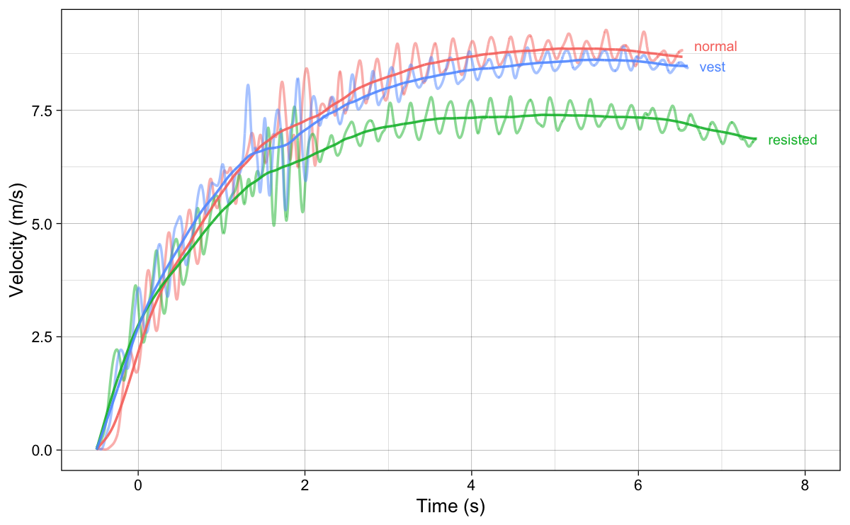
Figure 3: Laser gun data for a single individual. “Jumpy” lines represent the raw laser velocity, while the “smooth” line represent the smoothed velocity provided by the LaserSpeed device. Courtesy of Håkan Andresson
To avoid deceleration phase in the analysis, all three sprint traced are trimmed at 6s point. Mono-exponential model is fitted to each sprint using the {shorts} package (Jovanović and Vescovi 2022; Jovanović 2022) package (Figure 4).
Show/Hide Code
hakan <- hakan %>%
  filter(time <= 6)

# Get predictions
hakan <- hakan %>%
  group_by(type) %>%
  mutate(`velocity-predicted` = predict(model_radar_gun(time, `velocity-raw`))) %>%
  ungroup()

# Plot
ggplot(hakan, aes(x = time, color = type)) +
  theme_linedraw(8) +
  geom_line(aes(y = `velocity-raw`), alpha = 0.5) +
  geom_line(aes(y = `velocity-predicted`), alpha = 0.9) +
  geom_dl(
    aes(y = `velocity-predicted`, label = paste("  ", type)),
    method = list("last.bumpup", cex = 0.5)
  ) +
  xlim(-0.5, 6.5) +
  xlab("Time (s)") +
  ylab("Velocity (m/s)") +
  theme(legend.position = "none")
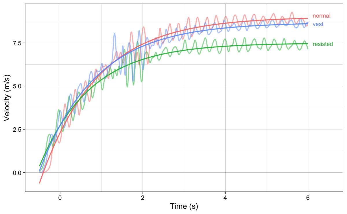
Figure 4: Predicted velocity using the models fitted with mono-exponential equation ({shorts} package (Jovanović and Vescovi 2022; Jovanović 2022) package)
The next step is to estimate the FVP using each individual sprint and the load conditions, as well as to estimate MSS and MAC for each condition assuming that the $F_0$ and $V_0$ from the normal sprint are mechanical determinants. In addition to this, I will provide estimated $F_0$ and $V_0$ disregarding the information about the load. Results are in Table 1.
Show/Hide Code
# Model
avp <- hakan %>%
  group_by(type) %>%
  summarise(data.frame(model_radar_gun(time, `velocity-raw`)$parameters)) %>%
  ungroup() %>%
  mutate(
    BW = athlete_BW,
    BH = athlete_BH,
    load = ifelse(type == "vest", vest_weight, 0),
    resistance = ifelse(type == "resisted", resistance, 0))

fvp <- avp %>%
  group_by(type) %>%
  mutate(find_FV(MSS, MAC, BW, BH, load, resistance)) %>%
  ungroup() %>%
  relocate(type, BW, BH) %>%
  select(-TC, -PMAX, -TAU)

# Created predicted sprint perf assuming normal F0 and V0 are "causal"
normal_fvp <- fvp %>%
  filter(type == "normal")

pred_avp <- function(df) {
  res <- find_AVP(normal_fvp$F0, normal_fvp$V0, df$BW, df$BH, df$load, df$resistance)

  data.frame(
    df,
    `predMSS` = res$MSS,
    `predMAC` = res$MAC)
}

disregard_cond <- function(df) {
  res <- find_FV(df$MSS, df$MAC, df$BW, df$BH, inertia = 0, resistance = 0)

  data.frame(
    df,
    `disregF0` = res$F0,
    `disregV0` = res$V0)
}

fvp <- fvp %>%
  rowwise() %>%
  do(pred_avp(.)) %>%
  do(disregard_cond(.))

kbl(fvp, digits = 2) %>%
  kable_classic(full_width = FALSE)
| type | BW | BH | MSS | MAC | load | resistance | F0 | V0 | predMSS | predMAC | disregF0 | disregV0 |
|---|---|---|---|---|---|---|---|---|---|---|---|---|
| normal | 82 | 1.86 | 9.01 | 6.52 | 0.0 | 0.00 | 534.57 | 9.45 | 9.01 | 6.52 | 534.57 | 9.45 |
| resisted | 82 | 1.86 | 7.49 | 6.05 | 0.0 | 64.75 | 560.71 | 8.82 | 7.92 | 5.73 | 495.96 | 7.76 |
| vest | 82 | 1.86 | 8.68 | 6.36 | 6.6 | 0.00 | 563.77 | 9.05 | 9.01 | 6.03 | 521.78 | 9.08 |
Table 1: Estimated sprint performance parameters (MSS and MAC) and FVP parameters (F0 and V0) for each sprint condition. predMSS and predMAC represent estimated sprint performance parameters assuming estimated $F_0$ and $V_0$ from a normal condition to be causal individual mechanical traits. disregF0 and disregV0 represent estimated FVP parameters disregarding information about additional load/resistance.
Let us discuss results from Table 1. When using only horizontal force resistance, theoretical model (Figure 2) predicts that both MSS and MAC will be affected. This is actually the case, as expected. But, the estimated $F_0$ and $V_0$ are not the same as those estimated with the normal sprint. If they are mechanical determinants, they should be equal (assuming there is no measurement error nor biological variation or fatigue/facilitation between sprints; that’s why we need more individuals). Estimated $F_0$ is actually larger than the $F_0$ estimated in the normal condition, which indicates that somehow, the individual is able to generate more initial horizontal force when using additional resistance. If $F_0$ is some type of the mechanical determinant, individual will show the same $F_0$, yielding smaller MAC, since part of it is spent on overcoming fixed horizontal resistance.
If we assume sprint FVP parameters estimated from the normal sprint condition to be mechanical determinants or traits, predicted MSS is larger than the observed, and predicted MAC is smaller than the observed (see Figure 5 for visual representation).
For the weighted vest condition, theoretical model (Figure 2) predicts that MAC will be affected, while MSS will stay the same. This is not the case (see Figure 5 for visual representation). Also, estimated $F_0$ is actually larger than the $F_0$ estimated in the normal condition, which indicates that somehow, the individual is able to generate more initial horizontal force when using additional inertia.
Show/Hide Code
pre_df <- fvp %>%
  filter(type == "normal") %>%
  select(MSS, MAC) %>%
  mutate(predMSS = MSS, predMAC = MAC, load = "norm") %>%
  expand_grid(type = c("resisted", "vest"))

post_df <- fvp %>%
  filter(type != "normal") %>%
  select(type, MSS, MAC, predMSS, predMAC) %>%
  mutate(load = "load")

df <- full_join(pre_df, post_df) %>%
  mutate(load = factor(load, levels = c("norm", "load")))

df_observed <- df %>%
  select(load, type, MSS, MAC) %>%
  pivot_longer(cols = c(MSS, MAC), names_to = "parameter") %>%
  mutate(model = "observed")

df_predicted <- df %>%
  select(load, type, predMSS, predMAC) %>%
  rename(MSS = predMSS,  MAC = predMAC) %>%
  pivot_longer(cols = c(MSS, MAC), names_to = "parameter") %>%
  mutate(model = "predicted")

plot_df <- rbind(df_observed, df_predicted) %>%
  mutate(parameter = factor(parameter, levels = c("MSS", "MAC")))

ggplot(plot_df, aes(x = load, y = value, color = model, group = model)) +
  theme_linedraw(8) +
  geom_line() +
  geom_point(fill = "white", shape = 21) +
  facet_grid(parameter~type, scales = "free") +
  geom_dl(
    aes(label = paste("  ", model)),
    method = list("last.bumpup", cex = 0.5)
  ) +
  xlab(NULL) +
  ylab(NULL) +
  theme(legend.position = "none")
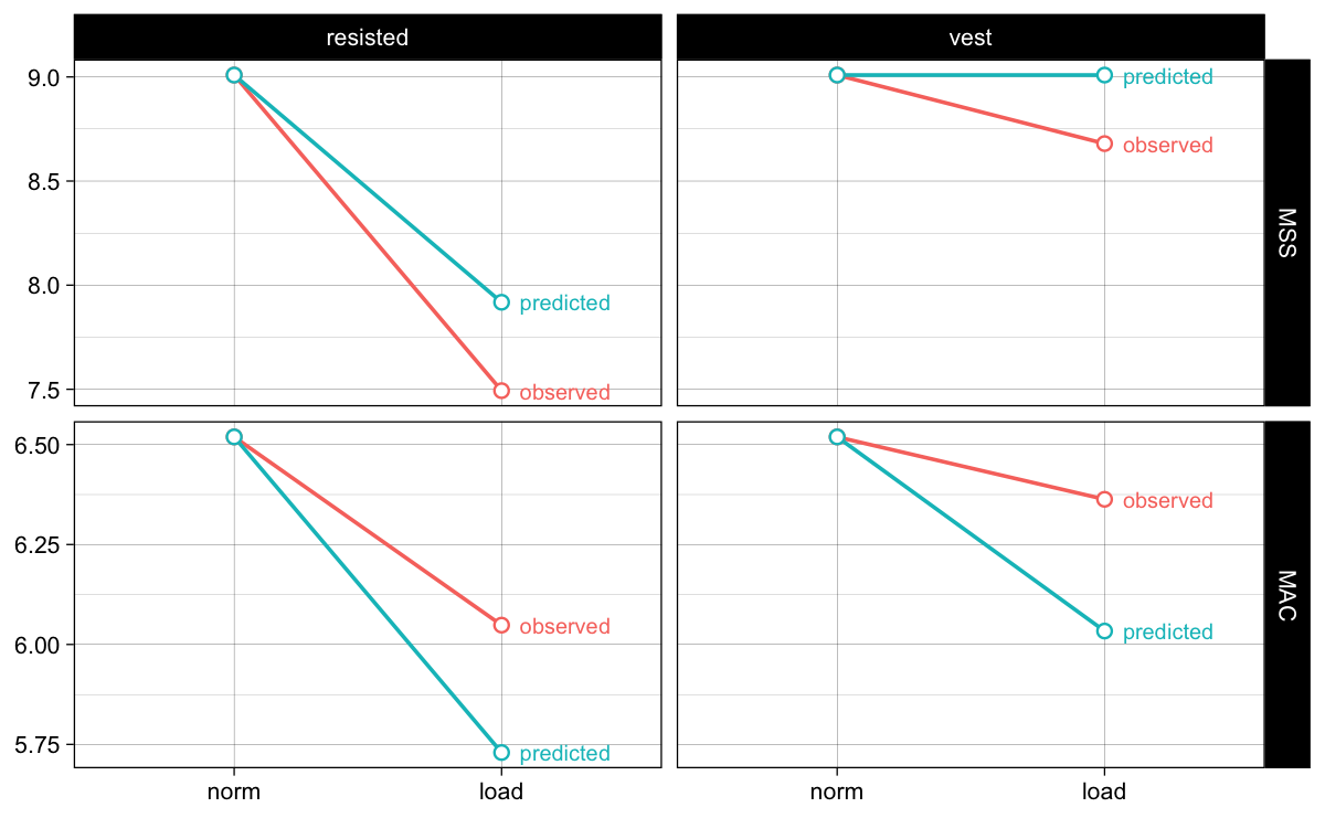
Figure 5: Comparisson between theoretical model sprint performance parameters predictions (i.e., assuming normal sprint estimated FVP parameters represent mechanical determinants or traits of the individual) and estimated sprint performance parameters
Although we need more samples, I do not think that this simple N=1 experiment support the realist model, which is implicit in viewing FVP as mechanical determinant of performance. Rather, I see FVP as additional performance summary (Figure 6) or indicators of performance that can pretty much be unnecessary if one knows MSS and MAC. Yeah, maybe one would like to know $F_0$ changes over time when individual also demonstrates changes in body weight, or if the ambient conditions change (e.g., air pressure, wind, or temperature) to check is someone “improved their force capabilities”, but this viewpoint actually takes the realist stance (with one being aware of it or not 1), that we have just disproved (assuming N=1 is enough to disprove it).
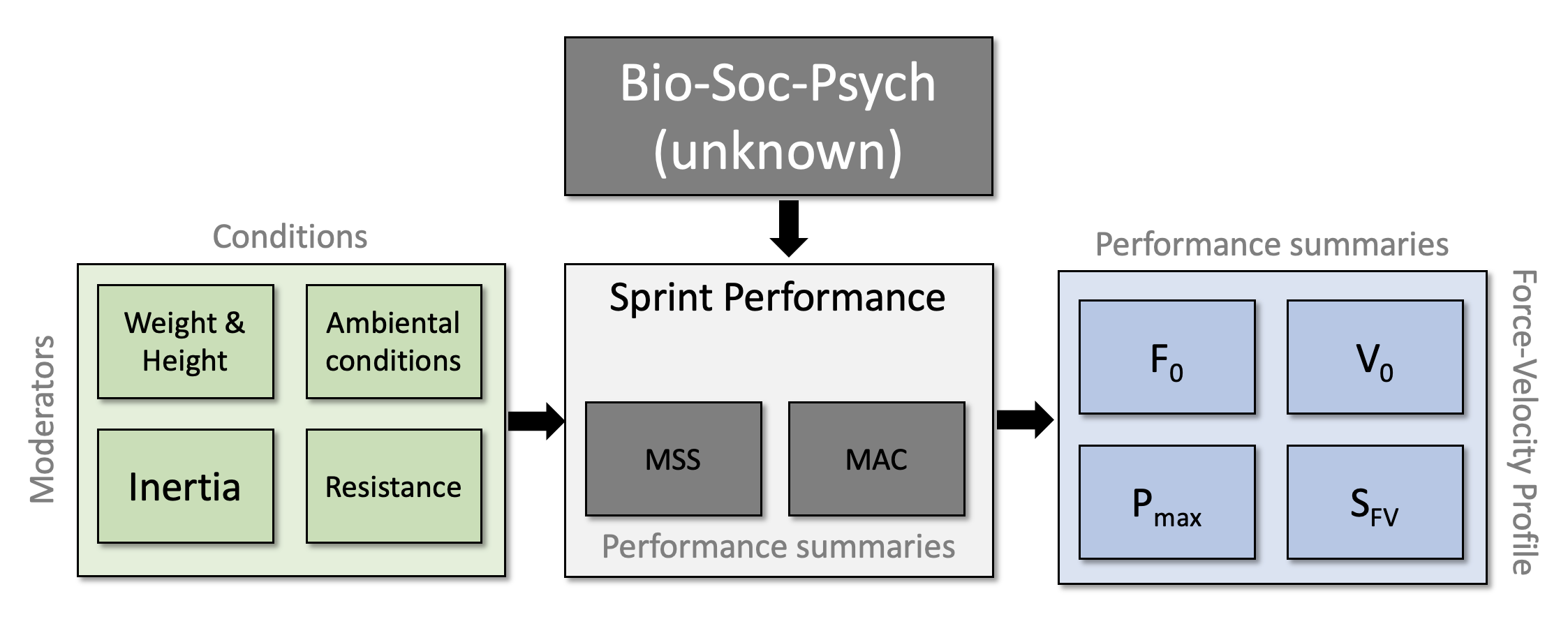
Figure 6: Instrumentalist viewpoint in which the $F_0$ and $V_0$ are simply indicators of performance
All in all, I still think that FVP is generally bollocks that seems to caught momentum and fame in the sports science community. It does looks like “science”, it does look like we are uncovering individual traits or qualities, especially will statements like “oh, your FVP profile is imbalanced – you need to work more on your ability to develop force” it is more pseudoscience maskarading as “evidence-based” scientific method. Am I against it? Yeah. I think summarizing sprint performance using MSS and MAC is enough. FVP will not give you anything more insightful or useful, except maybe to look and sound smart when presenting the data. Will you be able to pinpoint to performance limiter by looking at the FVP analysis? Nope. I still think that watching the sprint itself and motion-analysis will give you more information you might find actionable. For example, feet collapsing, or backside mechanics will not be seen in FVP profile. FVP profile will thus not determine sprint performance, but it will reflect sprint performance. If your fixing of someone’s feet collapsing or fixing someones back-side mechanics to be more front side improves sprint performance and thus FVP, then how can we state that FVP parameters represent mechanical determinants? Bollock, I tell you. Bollocks.
References
- Jovanović, Mladen. 2022. Shorts: Short Sprints. https://cran.r-project.org/package=shorts.
- Jovanović, Mladen, and Jason Vescovi. 2022. “Shorts: An r Package for Modeling Short Sprints.” International Journal of Strength and Conditioning 2 (1). https://doi.org/10.47206/ijsc.v2i1.74.
Footnotes
- Like it or not, or accept it or not, every our measurement, inference, or prediction assumes certain theoretical model. You just need to transparently state it, or if you are not aware of it, elucidate it. Eventually one can test predictions of such a model against the “real world” like we did in this installment. Yes we do need more samples to be conclusive, but this is a good start↩︎


Responses