Optimal Force-Velocity Profile for Sprinting: Is it all bollocks? – Part 2
Introduction
In the previous part I have introduced two models to map out velocity-time relationship in the short sprints. These models “simplify” the more complex (assumed) COM velocity trace when using the radar/laser gun, by providing “step-average” velocity. In this part I will focus on the characteristics of the mono-exponential model (Furusawa, Hill, and Parkinson 1927; Clark et al. 2017; P. Samozino et al. 2016a; Jovanović and Vescovi 2022).
As demonstrated in the previous part, the mono-exponential model better fits to our theoretical understanding and constraints of the short sprints, and also provides intuitive parameters to understand. In addition to this, mono-exponential model is mathematically “elegant”, and it can be integrated and differentiated to provide solution for modeling different types of short sprint data.
For example, radar/laser gun provides velocity time series. As such, one can use Equation 1 as model definition. Here the MSS represents the maximum sprinting speed and TAU represents relative acceleration. Mathematically, TAU represents the ratio of MSS to initial acceleration (MAC; maximal acceleration) (Equation 2). TAU can also be interpreted as the time required to reach a sprinting velocity equal to 63% of MSS. I personally favor the use of MSS and MAC, particularly since TAU seems to be around value of 1 s across various sports and athlete levels (Clark and Ryan 2022). This led some researchers to conclude that the acceleration and velocity performance limits are related and proportional (Clark and Ryan 2022). This is a topic for another article, but it is a direct counter-point to the concept of optimal FVP. I will come back to this later in this article series.
\begin{split}
v(t) = MSS \times (1 – e^{-\frac{t}{TAU}})\\\end{split}Equation 1
\begin{split}
MAC = \frac{MSS}{TAU}\\\end{split}Equation 2
If we differentiate Equation 1, we will get equation for acceleration (Equation 3). Elegantly, once we have estimated MSS and TAU parameters, mono-exponential equation allows us to predict kinematic and kinetic variables with ease.
\begin{split}
a(t) = \frac{MSS}{TAU} \times e^{-\frac{t}{TAU}}\\\end{split}Equation 3
Although radar/laser gun is considered the gold standard for estimating sprint profile (and also gives us the raw velocity trace that can be even more insightful than simple profile – see part one of this article series), we do not always have access to such technologies. More common alternative is using timing gates. With timing gates we do not get such a rich data set as with radar/laser gun, but we can still estimate MSS and TAU parameters. Integrating Equation 1 we get Equation 4, which we can use as model definition for the timing gates data.
\begin{split}
d(t) = MSS \times (t + TAU \times e^{-\frac{t}{TAU}}) – MSS \times TAU\\\end{split}Equation 4
Although one can use Equation 4, preferable model definition is Equation 5, since with timing gates, distance is predictor and the time is the outcome. It thus makes more statistical sense to model it as such.
\begin{split}
t(d) = TAU \times W(-e^{\frac{-d}{MSS \times TAU}} – 1) + \frac{d}{MSS} + TAU\\\end{split}Equation 5
If you are interested in how MSS and TAU are estimated using non-linear regression implemented in the {shorts} package, I suggest checking Jovanović and Vescovi (2022) and Jovanović (2022).
All in all, mono-exponential model is mathematically very simple and elegant and aligned with our theoretical model of short sprints: (1) sprint starts at $ t=0 $s, and (2) velocity reaches maximum without deceleration. There are few caveats with this, but it is beyond the scope of this article series (and it is the scope of my PhD thesis; you can read more about it in Jovanović and Vescovi (2022) and Jovanovic (2022)).
Kinematics and Acceleration-Velocity Profile
Once we have estimated MSS and TAU, be it from radar/laser gun velocity-time series, or from timing dates time-distance series, we can do all sort of wonderful things, like estimating kinematic and kinetic characteristics (again, step averaged – see previous part). This can be done across time or across distance, which can be more intuitive. Before we dig into the topic of optimal FVP, let us explore this further.
In the following examples we will assume mono-exponential model to be generative model (or data generating process; DGP). We will assume true MSS and TAU parameters, and use those to generate the data. We also do this when we estimate MSS and TAU from observed performance, but in that case we have additional noise, like time rounding, measurement error, performance variability, and so forth.
For the sake of exploration, we will utilize two athletes: Athlete A and Athlete B, for which we know the true values of MSS and TAU (Table 1).
Show/Hide Code
require(tidyverse)
require(shorts)
require(cowplot)
require(directlabels)
require(ggdist)
require(knitr)
require(kableExtra)

kbl(

tribble(~Athlete, ~MSS, ~TAU, ~MAC, ~PMAX,
          "Athlete A", 8, 1.33, 6, 12,
          "Athlete B", 6, 0.75, 8, 12)) %>%
  kable_classic(full_width = FALSE)
| Athlete | MSS | TAU | MAC | PMAX |
|---|---|---|---|---|
| Athlete A | 8 | 1.33 | 6 | 12 |
| Athlete B | 6 | 0.75 | 8 | 12 |
Table 1: Model generative parameter values for two hypothetical athletes with the same PMAX
Please note that the athletes in Table 1 have the same peak net relative power ($ P_{max} $, in W/kg), calculated using Equation 6.
\begin{split}
P_{max} = \frac{MSS \times MAC}{4}\\\end{split}Equation 6
Figure 1 depicts kinetic characteristics of the two athletes across sprint distance. Note that both athletes reach the same peak net relative power.
Show/Hide Code
athletes_df <- tribble(
  ~athlete, ~MSS, ~MAC,
  "Athlete A", 8, 6,
  "Athlete B", 6, 8
) %>%
  expand_grid(dist = seq(0, 40, length.out = 1000)) %>%
  mutate(
    `Time (s)` = predict_time_at_distance(dist, MSS, MAC),
    `Velocity (m/s)` = predict_velocity_at_distance(dist, MSS, MAC),
    `Acceleration (m/s/s)` = predict_acceleration_at_distance(dist, MSS, MAC),
    `Net Relative Power (W/kg)` = `Velocity (m/s)` * `Acceleration (m/s/s)`
  ) %>%
  pivot_longer(cols = c(`Time (s)`, `Velocity (m/s)`, `Acceleration (m/s/s)`, `Net Relative Power (W/kg)`), names_to = "variable") %>%
  mutate(variable = factor(variable, levels = c("Time (s)", "Velocity (m/s)", "Acceleration (m/s/s)", "Net Relative Power (W/kg)")))

ggplot(athletes_df, aes(x = dist, y = value, color = athlete)) +
  theme_linedraw(8) +
  geom_line(alpha = 0.8) +
  facet_wrap(~variable, scales = "free_y") +
  scale_color_brewer(palette = "Set1") +
  geom_dl(
    aes(label = paste("  ", athlete)),
    method = list("last.bumpup", cex = 0.5)
  ) +
  xlim(0, 50) +
  xlab("Distance (m)") +
  ylab(NULL) +
  theme(legend.position = "none")
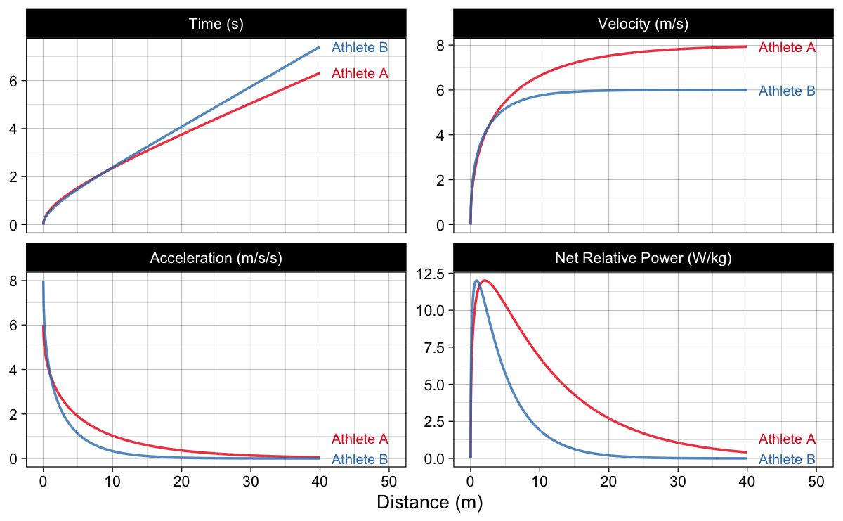
Figure 1: Kinematics using two hypothetical athletes. Please note that their Peak Net Relative Power (PMAX) is the same. One athlete is better “accelerator”, and the other has higher maximum sprinting speed.
If we plot (model-)predicted acceleration against (model-)predicted velocity, we will get Acceleration-Velocity Profile (AVP), which is, given the mono-exponential model, linear (Figure 2).
Show/Hide Code
athletes_avp_df <- athletes_df %>%
  filter(variable %in% c("Velocity (m/s)", "Acceleration (m/s/s)")) %>%
  pivot_wider(names_from = variable, values_from = value)

ggplot(athletes_avp_df, aes(x = `Velocity (m/s)`, y = `Acceleration (m/s/s)`, color = athlete)) +
  theme_linedraw(8) +
  geom_line(alpha = 0.8) +
  scale_color_brewer(palette = "Set1") +
  xlab("Velocity (m/s)") +
  ylab("Acceleration (m/s/s)") +
  geom_dl(
    aes(label = paste("  ", athlete)),
    method = list("last.bumpup", cex = 0.5)
  ) +
  theme(legend.position = "none") +
  xlim(0, 9)
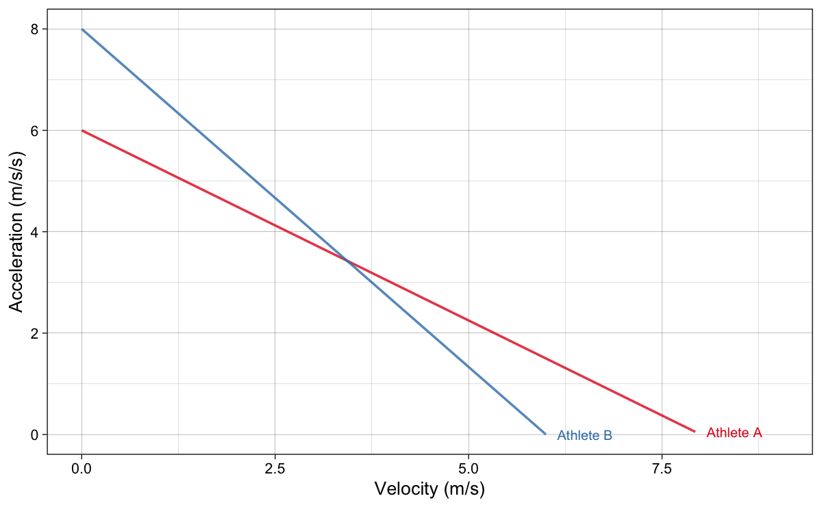
Figure 2: Acceleration-Velocity Profile
Please note that MSS is equal to the velocity value where the AVP crosses the x-axis, while MAC is equal to the acceleration value where the AVP crosses the y-axis. Slope of the curve can be expressed as Equation 7. It is interesting to note that the slope is also equal to negative TAU (Equation 8). Slope is interpreted as the decrease in acceleration (in $ ms^{-2} $) for every 1 $ ms^{-1} $ increase in velocity.
\begin{split}
S_{AV} = -\frac{MAC}{MSS}\\\end{split}Equation 7
\begin{split}
S_{AV} = -TAU\\\end{split}Equation 8
Kinetics and Force-Velocity Profile
To explore kinetics and Force-Velocity Profile (FVP), we will use two different athletes: Athlete C and Athlete D, which have the same sprint characteristics, but different body weight and body height (Table 2)
Show/Hide Code
athletes <- tribble(
  ~athlete, ~MSS, ~MAC, ~BW, ~Height,
  "Athlete C", 8, 8, 65, 1.65,
  "Athlete D", 8, 8, 105, 1.95
)


kbl(athletes) %>%
  kable_classic(full_width = FALSE)
| athlete | MSS | MAC | BW | Height |
|---|---|---|---|---|
| Athlete C | 8 | 8 | 65 | 1.65 |
| Athlete D | 8 | 8 | 105 | 1.95 |
Table 2: Model generative parameter values for two hypothetical athletes with the same sprint characteristics, but different body height and body weight
As explained in the previous part, we need to estimate air resistance force, that we can add to the $ m \times a $ to estimate total horizontal force, as well as power (this is power used to propel the body horizontally forward). Air force depends on the squared horizontal velocity and factor $ k $ (Equation 9). Factor $ k $ is a function of body weight, body height, air pressure, air temperature, and wind speed (please refer to Arsac and Locatelli (2002), P. Samozino et al. (2016b), and Ingen Schenau, Jacobs, and Koning (1991) for more information) (Equation 10).
\begin{split}
F_{air} = k \times v^2\\\end{split}Equation 9
\begin{split}
k = f(weight, \;height, \;Pressure, \;Temp, \;v_{wind})\\\end{split}Equation 10
If we know these parameters, and we know them as alluded in Table 2 (plus we use default 760 $ Torr $ air pressure, 25 $ C^\circ $ temperature, and zero wind velocity), we can estimate kinetics for our two athlete (Figure 3).
Show/Hide Code
athletes_df <-  athletes %>%
  expand_grid(dist = seq(0, 40, length.out = 1000)) %>%
  mutate(
    `Velocity (m/s)` = predict_velocity_at_distance(dist, MSS, MAC),
    `Air resistance (N)` = predict_air_resistance_at_distance(dist, MSS, MAC, bodymass = BW, bodyheight = Height),
    `Horizontal Force (N)` = predict_force_at_distance(dist, MSS, MAC, bodymass = BW, bodyheight = Height),
    `Relative Horizontal Force (N)` = `Horizontal Force (N)` / BW,
    `Power (W)` = predict_power_at_distance(dist, MSS, MAC, bodymass = BW, bodyheight = Height),
    `Relative Power (W/kg)` = `Power (W)` / BW
  ) %>%
  pivot_longer(cols = c(`Velocity (m/s)`, `Air resistance (N)`, `Horizontal Force (N)`, `Relative Horizontal Force (N)`, `Power (W)`, `Relative Power (W/kg)`), names_to = "variable") %>%
  mutate(variable = factor(variable, levels = c("Velocity (m/s)", "Air resistance (N)", "Horizontal Force (N)", "Relative Horizontal Force (N)", "Power (W)", "Relative Power (W/kg)")))


ggplot(athletes_df, aes(x = dist, y = value, color = athlete)) +
  theme_linedraw(8) +
  geom_line(alpha = 0.8) +
  facet_wrap(~variable, scales = "free_y") +
  scale_color_brewer(palette = "Set1") +
  geom_dl(
    aes(label = paste("  ", athlete)),
    method = list("last.bumpup", cex = 0.5)
  ) +
  xlim(0, 55) +
  xlab("Distance (m)") +
  ylab(NULL) +
  theme(legend.position = "none")
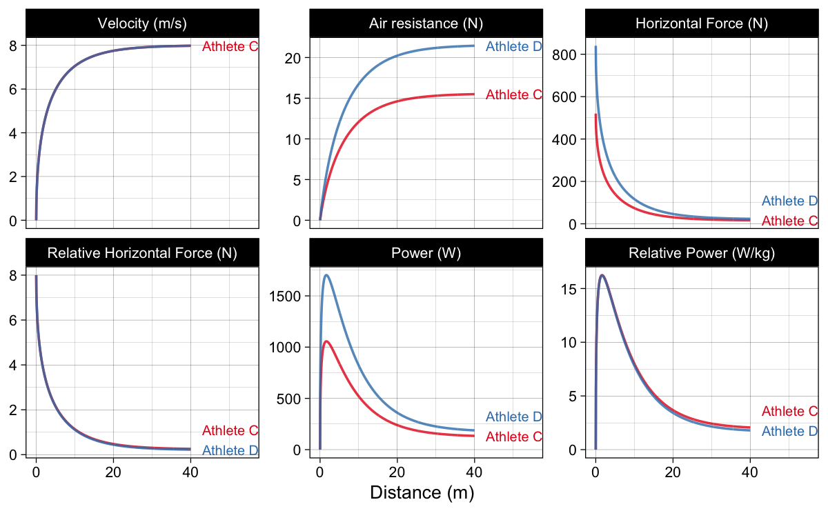
Figure 3: Kinetic variables. Here we assume that the Athlete C weights 65kg and has 165cm of height, while Athlete D weights 105kg and has 195cm of height
As can be seen from Figure 3, kinematic characteristics for Athlete C and Athlete D are equal (i.e., same velocity trace, and thus same acceleration, and relative net power), but kinematic characteristics are different due to different air resistance and body mass.
If we plot the estimated horizontal force and estimated relative horizontal force against estimated velocity, we will get Force-Velocity Profile (Figure 4).
Show/Hide Code
athletes_FVP_df <- athletes_df %>%
  filter(variable %in% c("Velocity (m/s)", "Horizontal Force (N)", "Relative Horizontal Force (N)")) %>%
  pivot_wider(names_from = variable, values_from = value) %>%
  pivot_longer(cols = c(`Horizontal Force (N)`, `Relative Horizontal Force (N)`), names_to = "variable")

ggplot(athletes_FVP_df, aes(x = `Velocity (m/s)`, y = value, color = athlete)) +
  theme_linedraw(8) +
  geom_line(alpha = 0.8) +
  scale_color_brewer(palette = "Set1") +
  xlab("Velocity (m/s)") +
  ylab(NULL) +
  geom_dl(
    aes(label = paste("  ", athlete)),
    method = list("last.bumpup", cex = 0.5)
  ) +
  theme(legend.position = "none") +
  xlim(0, 9.5) +
  facet_wrap(~variable, scales = "free_y")
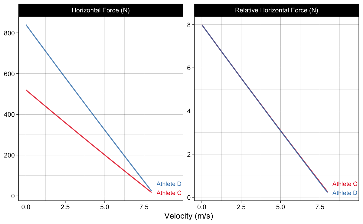
Figure 4: Force-Velocity Profile
We can summarize FVP by estimating (or calculating) $ F_0 $ (can be either absolute, or relative) and $ V_0 $. This can be done by simply fitting a linear regression line to the estimated FV trace (Equation 11).
\begin{split}
F = b_0 + b_1 \times v\\\end{split}Equation 11
Using estimated regression parameters $ b_0 $ and $ b_1 $ we can estimate $ F_0 $ and $ V_0 $ (Equation 12 and Equation 13).
\begin{split}
F_0 = b_0\\\end{split}Equation 12
\begin{split}
V_0 = -\frac{b_0}{b_1}\\\end{split}Equation 13
Due to air resistance involved, this FVP is not linear (as opposed to the AVP). This can be seen when plotting residuals (Figure 5), or you can tilt your screen and check the Figure 4.
Show/Hide Code
get_resid <- function(.x) {
  m1 <- lm(value ~ `Velocity (m/s)`, .x)
  .x$resid <- resid(m1)
  .x$fitted <- fitted(m1)
  .x
}

athletes_FVP_df <- athletes_FVP_df  %>%
  group_by(athlete, variable) %>%
  do(get_resid(.)) %>%
  ungroup

ggplot(athletes_FVP_df, aes(x = `Velocity (m/s)`, y = resid, color = athlete)) +
  theme_linedraw(8) +
  geom_hline(yintercept = 0, linetype = "dotted") +
  geom_line(alpha = 0.8) +
  scale_color_brewer(palette = "Set1") +
  xlab("Velocity (m/s)") +
  ylab("Residual") +
  geom_dl(
    aes(label = paste("  ", athlete)),
    method = list("last.bumpup", cex = 0.5)
  ) +
  theme(legend.position = "none") +
  xlim(0, 9) +
  facet_wrap(~variable, scales = "free_y")
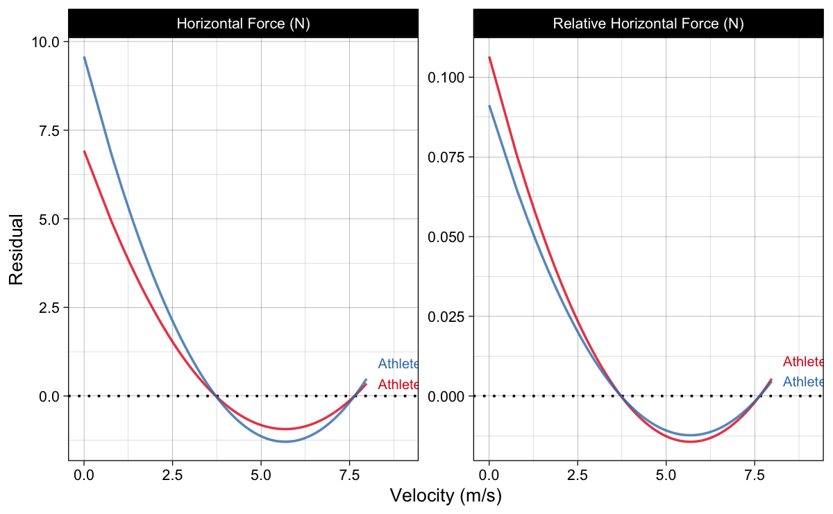
Figure 5: Force-Velocity Profile residuals
Another method of estimating $ F_0 $ and $ V_0 $ is through calculus, named polynomial method (see Pierre Samozino et al. (2022) for more details) (Equation 14 and Equation 15).
\begin{split}
F_0 = MAC \times BW\\\end{split}Equation 14
\begin{split}
V_0 = \frac{1}{2 \times k \times TAU} \times (1 – \sqrt{1 – 4 \times k \times MSS})\\\end{split}Equation 15
Table 3 contains estimated $ F_0 $ and $ V_0 $ using two methods for Athlete C and Athlete D. As you can notice, they differ slightly. I will explore these difference using simple simulation shortly. Prefered method is of course using the polynomial method.
Show/Hide Code
athletes_FVP <- athletes %>%
  rowwise() %>%
  mutate(
    data.frame(make_FV_profile(MSS, MAC, bodymass = BW, bodyheight = Height)[c("F0", "F0_rel", "V0", "F0_poly", "F0_poly_rel", "V0_poly")])
  )

kbl(athletes_FVP, digits = 2) %>%
  kable_classic(full_width = FALSE)
| athlete | MSS | MAC | BW | Height | F0 | F0_rel | V0 | F0_poly | F0_poly_rel | V0_poly |
|---|---|---|---|---|---|---|---|---|---|---|
| Athlete C | 8 | 8 | 65 | 1.65 | 515.50 | 7.93 | 8.24 | 520 | 8 | 8.26 |
| Athlete D | 8 | 8 | 105 | 1.95 | 833.77 | 7.94 | 8.20 | 840 | 8 | 8.22 |
Table 3: Estimated F0 and V0 using two methods for Athletes C and D
Another way to summarize the FVP is to use slope ($ S_{FV} $) (Equation 16) and max power ($ P_{max} $) (Equation 17). This is done using using relative $ F_0 $.
\begin{split}
S_{FV} = -\frac{F_0}{V_0}\\\end{split}Equation 16
\begin{split}
P_{max} = \frac{F_0 \times V_0}{4}\\\end{split}Equation 17
Using $ P_{max} $ and $ S_{FV} $ one can reverse-engineer the math to get the equation for the time at distance (Equation 18) (see Pierre Samozino et al. (2022) for more details)
\begin{split}
t(d) = f(d, \; P_{max}, \; S_{FV}, \; k)\\\end{split}Equation 18
And this is, ladies and gentlemen, the basis of the Optimal FVP model for sprinting. In short, it assumes that P_{max} is some type of determinant of performance (although it has been estimated from performance itself), while we can shift the $ S_{FV} $ to minimize the time it takes to cover specific distance. I will explore this in much more details in the next installment of this article series.
Quick simulation
Due to not-exactly-linear FV relationship (Figure 4 and Figure 5), peak power ($ P_{peak} $) will differ from $ P_{max} $, estimated using Equation 17 (Figure 6).
Show/Hide Code
athletes_power <- athletes %>%
  rowwise() %>%
  mutate(
    data.frame(make_FV_profile(MSS, MAC, bodymass = BW, bodyheight = Height)[c("Pmax_poly", "Pmax_poly_rel")])
  ) %>%
  ungroup() %>%
  rename(`Relative Power (W/kg)` = Pmax_poly_rel, `Power (W)` = Pmax_poly) %>%
  pivot_longer(cols = c("Power (W)", "Relative Power (W/kg)"), names_to = "variable", values_to = "value")

athletes_df %>%
  filter(
    variable %in% c("Power (W)", "Relative Power (W/kg)"),
    dist < 15) %>%
ggplot(aes(x = dist, y = value, color = athlete)) +
  theme_linedraw(8) +
  geom_line(alpha = 0.8) +
  geom_hline(data = athletes_power, aes(yintercept = value, color = athlete), linetype = "dashed") +
  facet_wrap(~variable, scales = "free_y") +
  scale_color_brewer(palette = "Set1") +
  geom_dl(
    aes(label = paste("  ", athlete)),
    method = list("last.bumpup", cex = 0.5)
  ) +
  xlim(0, 20) +
  xlab("Distance (m)") +
  ylab(NULL) +
  theme(legend.position = "none")
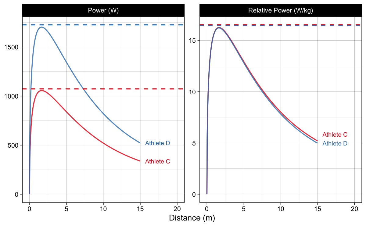
Figure 6: Differences bewteen estimated Pmax and Ppeak. Dashed line represents individual athlete Pmax
It is thus important to realize that $ P_{max} $ estimated using Equation 17 is just a quick proxy, and thus biased method, to estimate model $ P_{peak} $. In contrast, net relative $ P_{max} $ and $ P_{peak} $ are exactly the same for the AVP. This is not the case for the FVP due to air resistance.
To explore these differences between two methods (using regression and using polynomial) to estimate $ F_0 $ and $ V_0 $, and thus $ S_{FV} $ and $ P_{max} $, as well the difference between polynomially estimated $ P_{max} $ and $ P_{peak} $, I will utilize a simple simulation.
We are going to simulate a range of true MSS values (from 6 to 11 $ ms^{-1} $), TAU values (from 0.9 to 1.1 $ s $), and body weight (from 65 to 105 kg; assuming height of 1.75 m) and then estimate the aforementioned parameters and calculate percent difference between them using Equation 19.
\begin{split}
\%Diff = 100 \times \frac{x_1 – x_2}{\frac{x_1 + x_2}{2}}\\\end{split}Equation 19
Figure 7 depicts distribution of the percent differences. These differences are not large, but they are still involved and can cause bias later when optimizing the FVP. Even if this bias is negligent, we are still puzzled with which parameter to utilize when optimizing the FVP. I will explore these topics in the next installment.
Show/Hide Code
perc_diff <- function(x1, x2) {
  100 * (x1 - x2) / ((x1 + x2) / 2)
}

sim_df <- expand_grid(
  MSS = seq(6, 11, length.out = 10),
  TAU = seq(0.9, 1.1, length.out = 10),
  BW = seq(65, 105, length.out = 10)
) %>%
  mutate(MAC = MSS / TAU) %>%
  rowwise() %>%
  mutate(as.data.frame(make_FV_profile(MSS = MSS, MAC = MAC, bodymass = BW)[c("F0", "F0_rel", "F0_poly", "F0_poly_rel", "V0", "V0_poly", "Pmax", "Pmax_rel", "Pmax_poly", "Pmax_poly_rel", "FV_slope", "FV_slope_poly")])) %>%
  mutate(
    Ppeak = find_max_power_time(MSS, MAC, bodymass = BW)[[1]],
    Ppeak_rel = Ppeak / BW
  ) %>%
  ungroup()


sim_df_summary <- sim_df %>%
  mutate(
    `V0 diff (%)` = perc_diff(V0, V0_poly),
    `F0 diff (%)` = perc_diff(F0, F0_poly),
    `Slope diff (%)` = perc_diff(FV_slope, FV_slope_poly),
    `Pmax diff (%)` = perc_diff(Pmax, Pmax_poly),
    `Power diff (%)` = perc_diff(Pmax_poly, Ppeak)
  ) %>%
  select(`V0 diff (%)`, `F0 diff (%)`, `Slope diff (%)`, `Pmax diff (%)`, `Power diff (%)`) %>%
  pivot_longer(cols = c(`V0 diff (%)`, `F0 diff (%)`, `Slope diff (%)`, `Pmax diff (%)`, `Power diff (%)`), names_to = "variable") %>%
  mutate(variable = factor(variable, levels = c("V0 diff (%)", "F0 diff (%)", "Slope diff (%)", "Pmax diff (%)", "Power diff (%)")))

ggplot(sim_df_summary, aes(x = variable, y = value, fill = variable)) +
  theme_linedraw(8) +
  geom_hline(yintercept = 0, linetype = "dotted") +
  ggdist::stat_halfeye(alpha = 0.7, trim = FALSE, normalize = "groups", scale = 0.8, .width = 0.9) +
  scale_fill_brewer(palette = "Set1") +
  xlab(NULL) +
  ylab("% Difference") +
  theme(legend.position = "none")
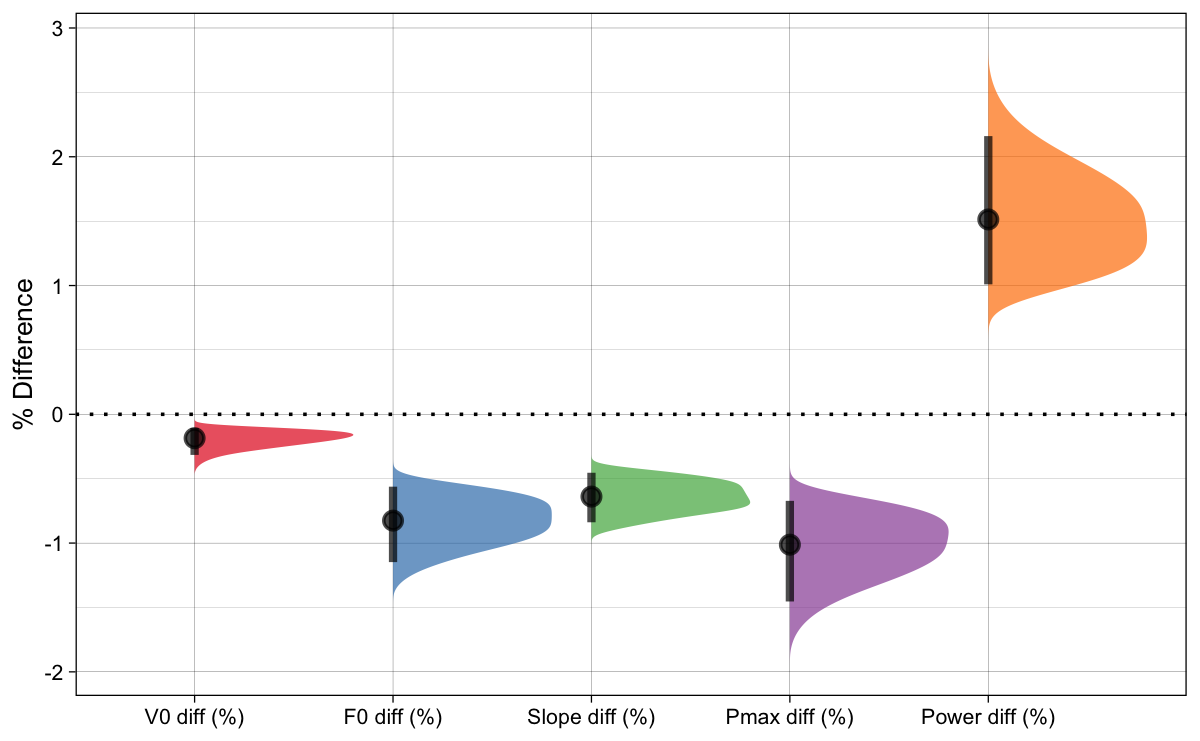
Figure 7: Percent Difference using simulation
Summary
In this part of article series, we have explored the behavior of the mono-exponential model, as well as some different ways to summarize the estimated FVP. Please read this again – we have explored the behavior of the MODEL, not of the athletes (Figure 8). I have a beef with calling $ F_0 $, $ V_0 $, or $ P_{max} $ and $ S_{FV} $ determinants of performance since they are estimated from performance itself. If the performance improves, these parameters will improve as well, and not vice versa. Yet, to accept the optimization of the FVP for the sake of intervention, one needs to take the realist perspective and assume $ P_{max} $ and $ S_{FV} $ are real traits of the athlete (i.e., determinants of performance). You can read my discussion with Pierre Samozino on Twitter on this very topic here and here.
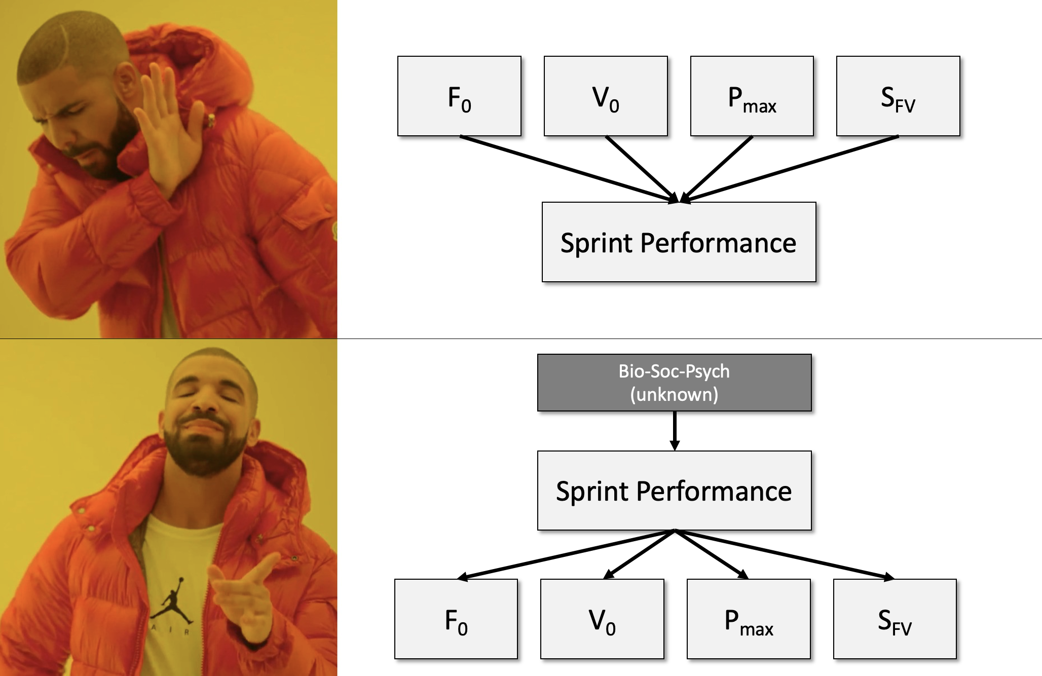
Figure 8: Even Drake doesn’t like the realist/reflective causal model, and prefers the constructionist/formative model with unknown true causes. Read more about this in Jovanović (2020)
I will explore the concept of optimization in the next installment. It is important not to confuse the map for the territory.
References
- Arsac, Laurent M., and Elio Locatelli. 2002. “Modeling the Energetics of 100-m Running by Using Speed Curves of World Champions.” Journal of Applied Physiology 92 (5): 1781–88. https://doi.org/10.1152/japplphysiol.00754.2001.
- Clark, Kenneth P., Randall H. Rieger, Richard F. Bruno, and David J. Stearne. 2017. “The NFL Combine 40-Yard Dash: How Important Is Maximum Velocity?” Journal of Strength and Conditioning Research, June, 1. https://doi.org/10.1519/JSC.0000000000002081.
- Clark, Kenneth P., and Laurence J. Ryan. 2022. “Hip Torque Is a Mechanistic Link Between Sprint Acceleration and Maximum Velocity Performance: A Theoretical Perspective.” Frontiers in Sports and Active Living 4 (July): 945688. https://doi.org/10.3389/fspor.2022.945688.
- Furusawa, K., Archibald Vivian Hill, and J. L. Parkinson. 1927. “The Dynamics of "Sprint" Running.” Proceedings of the Royal Society of London. Series B, Containing Papers of a Biological Character 102 (713): 29–42. https://doi.org/10.1098/rspb.1927.0035.
- Ingen Schenau, Gerrit Jan van, Ron Jacobs, and Jos J. de Koning. 1991. “Can Cycle Power Predict Sprint Running Performance?” European Journal of Applied Physiology and Occupational Physiology 63 (3-4): 255–60. https://doi.org/10.1007/BF00233857.
- Jovanovic, Mladen. 2022. “Bias in Estimated Short Sprint Profiles Using Timing Gates Due to the Flying Start: Simulation Study and Proposed Solutions.” https://doi.org/10.51224/SRXIV.179.
- Jovanović, Mladen. 2020. Strength Training Manual: The Agile Periodization Approach. Independently published.
- ———. 2022. Shorts: Short Sprints. https://cran.r-project.org/package=shorts.
- Jovanović, Mladen, and Jason Vescovi. 2022. “Shorts: An r Package for Modeling Short Sprints.” International Journal of Strength and Conditioning 2 (1). https://doi.org/10.47206/ijsc.v2i1.74.
- Samozino, Pierre, Nicolas Peyrot, Pascal Edouard, Ryu Nagahara, Pedro Jimenez-Reyes, Benedicte Vanwanseele, and Jean-Benoit Morin. 2022. “Optimal Mechanical Force–Velocity Profile for Sprint Acceleration Performance.” Scandinavian Journal of Medicine & Science in Sports 32 (3): 559–75. https://doi.org/10.1111/sms.14097.
- Samozino, P., G. Rabita, S. Dorel, J. Slawinski, N. Peyrot, E. Saez de Villarreal, and J.-B. Morin. 2016b. “A Simple Method for Measuring Power, Force, Velocity Properties, and Mechanical Effectiveness in Sprint Running: Simple Method to Compute Sprint Mechanics.” Scandinavian Journal of Medicine & Science in Sports 26 (6): 648–58. https://doi.org/10.1111/sms.12490.
- ———. 2016a. “A Simple Method for Measuring Power, Force, Velocity Properties, and Mechanical Effectiveness in Sprint Running: Simple Method to Compute Sprint Mechanics.” Scandinavian Journal of Medicine & Science in Sports 26 (6): 648–58. https://doi.org/10.1111/sms.12490.


Responses