Non-responders: are they really?
Introduction
Latest obsesion of the researches is individual variation in training responses. The motivation behind this approach (known and emphasized in theory of training as individualization principle) is the creation of personalized medicine or personalized training.
Unfortunately, sometimes we see these individual differences (in treatment reaction), although they are artefacts of within-individual typical variation/error of measurement and regression to the mean.
These are the very important concepts discussed in great paper by Atkinson and Batterham in Journal of Experimental Physiology (2015, ahead of print). I highly urge you to read it before proceeding with the following simulation of mine.
Problem
Without scaring the non-statistically inclined readers, I will use very simple example from real life. We are interested in effects of one training + diet intervention on body weight BW of our subjects, and whether we can identify the responders vs. non-responders.
If there are responders and non-responders, we might be interested in what other variable can predict it (using mediation/moderation analysis, ANCOVA, mixed-models and so forth – please note that I am not that versed in these yet).
It is important to state, in my opinion there are no general responders and non-responders – they are related to intervention at hand (although there might be individuals who are genetically more lucky in general – hence they response positively to anything thrown at them).
Let’s assume we recruited 200 participants, with “real” body weight of 100kg and around 15kg between-individual SD.
library(ggplot2)
library(reshape2)

set.seed(1107) # Set the random number seed so you can replicate the data

n.subjects <- 200

# Generate our sample
pre.subjects.real.BW <- rnorm(mean = 100,
                              sd = 15,
                              n = n.subjects)

# Plot histogram
gg <- ggplot(data.frame(BW = pre.subjects.real.BW), aes(x = BW))
gg <- gg + geom_density(fill = "grey", alpha = 0.4)
gg <- gg + theme_bw()
gg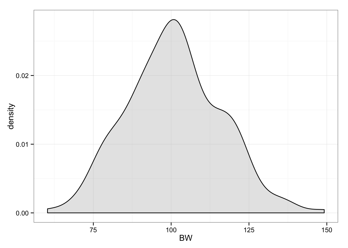
Now we randomly split them into two groups (n = 100): Intervention and Control
# Generate 100 random numbers (uniformly)
group.index <- sample(1:n.subjects, n.subjects / 2)

# Pull out intervention subjects
pre.intervention.real.BW <- pre.subjects.real.BW[group.index]

# Pull out control subjects
pre.control.real.BW <- pre.subjects.real.BW[-group.index]

# Create data frame for plotting
df <- data.frame(intervention = pre.intervention.real.BW,
                 control = pre.control.real.BW)

# Reshape for ggplot
df <- melt(df,
           id.vars = NULL,
           variable.name = "Group",
           value.name = "BW")

# Plot
gg <- ggplot(df, aes(x = BW, fill = Group))
gg <- gg + geom_density(alpha = 0.4)
gg <- gg + theme_bw()
gg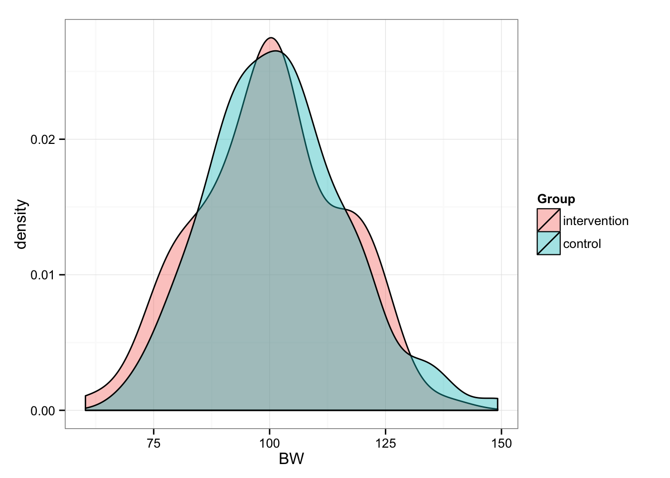
# And summary statistics
summary(pre.intervention.real.BW)
## Min. 1st Qu. Median Mean 3rd Qu. Max.
## 60.28 89.62 100.30 100.00 110.50 138.00summary(pre.control.real.BW)## Min. 1st Qu. Median Mean 3rd Qu. Max.
## 69.56 92.16 101.50 101.80 110.20 149.20Now we have two equal groups of n = 100, BW = 100 (15). But before we proceed, let’s deal with “real” BW. In this case “true” refers to “true” bodyweight of the subject. But as we know any measure varies because of measurement error and biological variability (i.e. noise). For example, if my “real” bodyweight is 95kg, due normal biological fluctuations and my scale error I might score 94-96kg on different days.
Let’s assume (we should measure the reliability of our metrics, but for the sake of this simulation we assume) that our typical variation is 0.5 kg and it is normally distributed. This means that in 95% of times, any single subject weight will fluctuate between -1 and +1 kg.
So let’s apply this typical variation to our pre- bodyweights.
# Create a simple function that creates typical variation
TV <- 0.5
typical.var <- function(SD = TV, n = n.subjects / 2) {
    return(rnorm(mean = 0, sd = SD, n))
}

# Add typical variation or noise
pre.intervention.measured.BW <- pre.intervention.real.BW + typical.var()
pre.control.measured.BW <- pre.control.real.BW + typical.var()

# Create data frame for plotting
pre <- data.frame(intervention = pre.intervention.measured.BW,
                 control = pre.control.measured.BW)

# Reshape for ggplot
pre <- melt(pre,
           id.vars = NULL,
           variable.name = "Group",
           value.name = "Measured.BW")

# Plot
gg <- ggplot(pre, aes(x = Measured.BW, fill = Group))
gg <- gg + geom_density(alpha = 0.4)
gg <- gg + theme_bw()
gg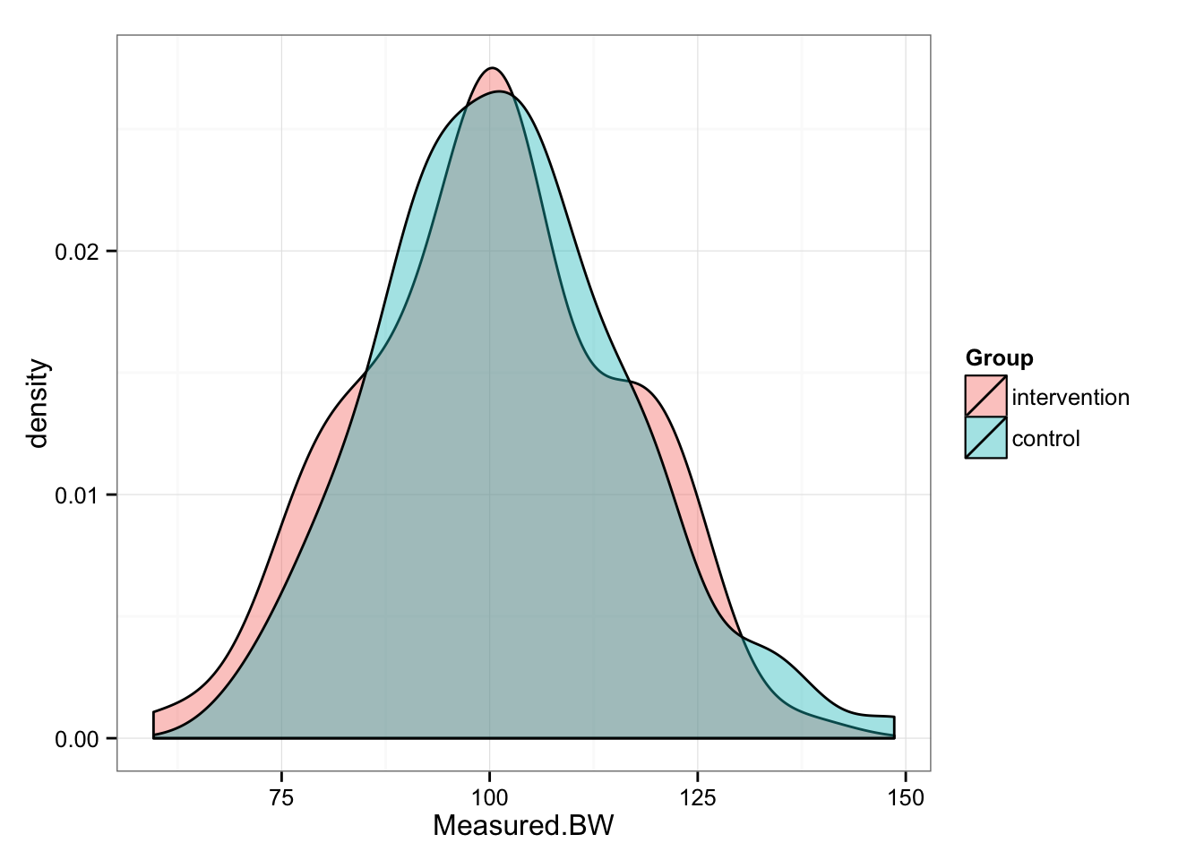
# And summary statistics
summary(pre.intervention.measured.BW)
## Min. 1st Qu. Median Mean 3rd Qu. Max.
## 59.60 89.35 100.40 100.00 110.30 138.10summary(pre.control.measured.BW)## Min. 1st Qu. Median Mean 3rd Qu. Max.
## 69.46 92.10 101.40 101.90 110.30 148.60We can perform t test to confirm that our groups in pre- conditions are identical
t.test(pre.intervention.measured.BW,
       pre.control.measured.BW)
##
## Welch Two Sample t-test
##
## data: pre.intervention.measured.BW and pre.control.measured.BW
## t = -0.883, df = 197.918, p-value = 0.3783
## alternative hypothesis: true difference in means is not equal to 0
## 95 percent confidence interval:
## -6.063432 2.312780
## sample estimates:
## mean of x mean of y
## 99.9953 101.8706Let’s assume that the “real” change in Intervention group is 3 kg – in other words all subjects that were in intervention group reduced their “real” BW for 3 kg. In this case 3 kg represents smallest worthwhile change (SWC).
The control group experienced 0 (zero) change in “real” bodyweight, hence no effect.
But, since we are measuring post- bodyweight as well, we are again introducing typical variation. Let’s calculate post- real and measured bodyweight for both groups
# the "real" change of 3 kg in intervention group
post.intervention.real.BW <- pre.intervention.real.BW - 3

# No "real" change in control group
post.control.real.BW <- pre.control.real.BW - 0

# Now let's calculate "measures" post- bodyweights by adding typical variation
post.intervention.measured.BW <- post.intervention.real.BW + typical.var()
post.control.measured.BW <- post.control.real.BW + typical.var()


# Create data frame for plotting
post <- data.frame(intervention = post.intervention.measured.BW,
                 control = post.control.measured.BW)

# Reshape for ggplot
post <- melt(post,
           id.vars = NULL,
           variable.name = "Group",
           value.name = "Measured.BW")

# Plot
gg <- ggplot(post, aes(x = Measured.BW, fill = Group))
gg <- gg + geom_density(alpha = 0.4)
gg <- gg + theme_bw()
gg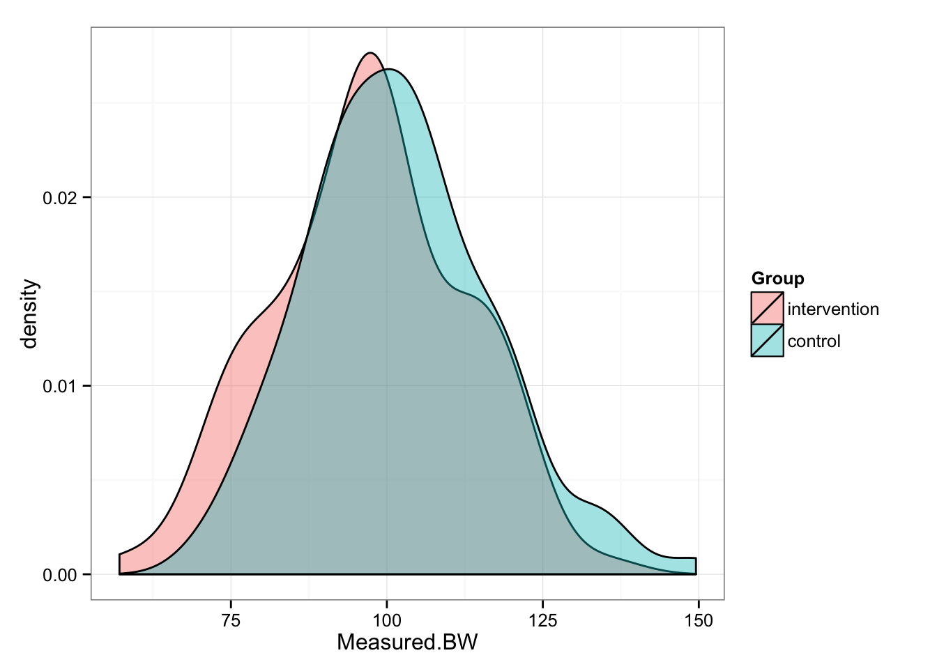
# And summary statistics
summary(post.intervention.measured.BW)
## Min. 1st Qu. Median Mean 3rd Qu. Max.
## 57.13 87.11 97.52 96.97 107.30 135.60summary(post.control.measured.BW)## Min. 1st Qu. Median Mean 3rd Qu. Max.
## 69.71 92.13 101.40 101.90 110.40 149.50Let’s create trellis plot and plot pre/post for Intervention and Control groups
pre$Period <- "Pre"
post$Period <- "Post"

# Concatenate the data framaes
experiment.data <- rbind(pre, post)
experiment.data$Period <- factor(experiment.data$Period,
                                levels = c("Pre", "Post"))

# Plot
gg <- ggplot(experiment.data, aes(x = Measured.BW, fill = Period))
gg <- gg + geom_density(alpha = 0.4)
gg <- gg + theme_bw()
gg <- gg + facet_wrap(~Group)
gg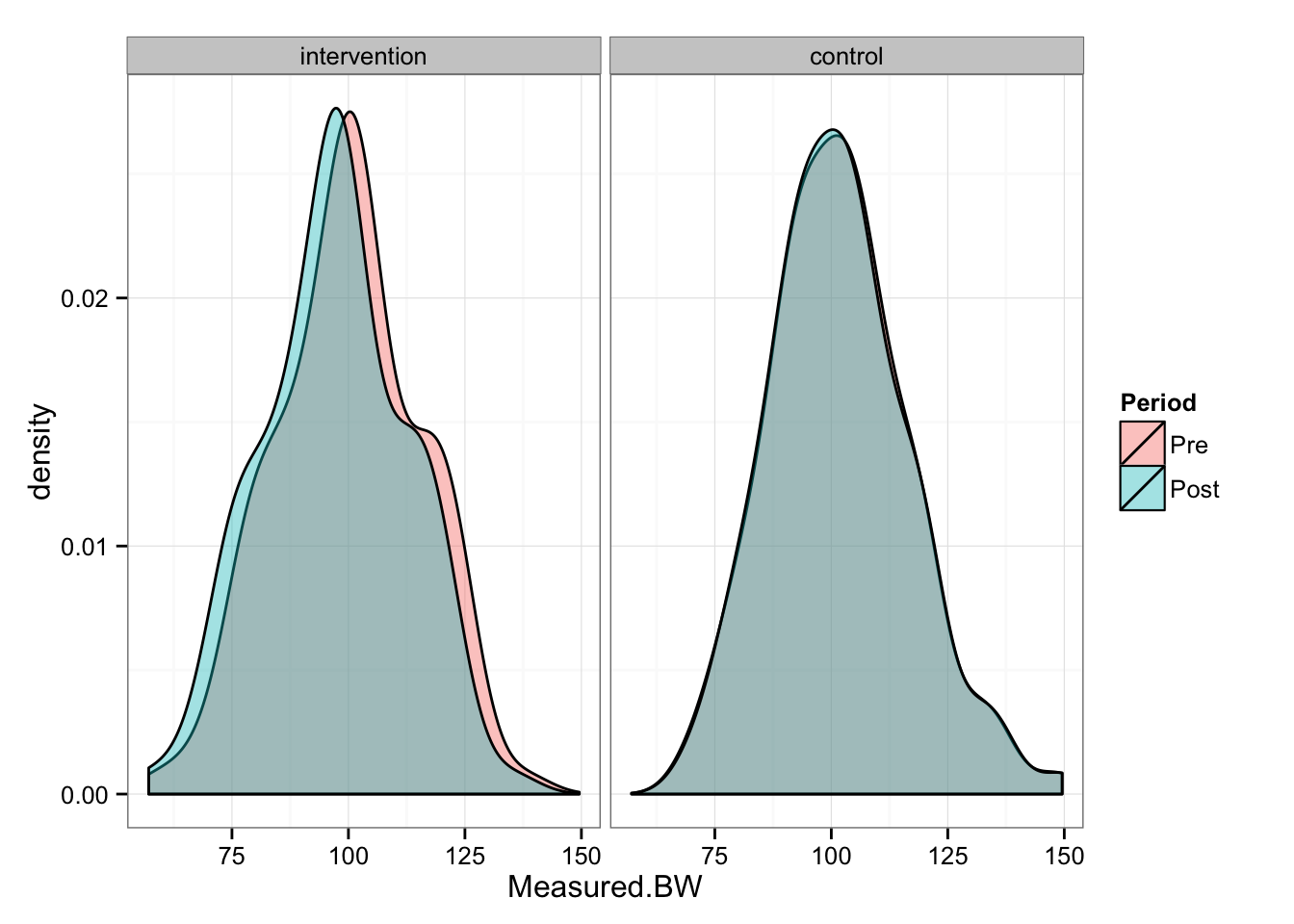
As can be seen from the picture, Intervention group “shifted” for 3 kg, while Control group stayed the same. We can perform paired (repeated-measures) t test to check the differences in the groups between pre- and post-
# Intervention group
t.test(pre.intervention.measured.BW,
       post.intervention.measured.BW,
       paired = TRUE)
##
## Paired t-test
##
## data: pre.intervention.measured.BW and post.intervention.measured.BW
## t = 45.6962, df = 99, p-value < 2.2e-16
## alternative hypothesis: true difference in means is not equal to 0
## 95 percent confidence interval:
## 2.893269 3.155937
## sample estimates:
## mean of the differences
## 3.024603# Control gorup
t.test(pre.control.measured.BW,
post.control.measured.BW,
paired = TRUE)##
## Paired t-test
##
## data: pre.control.measured.BW and post.control.measured.BW
## t = 0.2393, df = 99, p-value = 0.8114
## alternative hypothesis: true difference in means is not equal to 0
## 95 percent confidence interval:
## -0.1125848 0.1434657
## sample estimates:
## mean of the differences
## 0.01544046As can be seen from the t test, Control group had statistically not significant change, while Intervention group had statistically significant change.
Since we know (because this is simulation) that the “real” change in Intervention group for EVERY subject is 3kg, let’s plot the measured change in bodyweight. On the following graph, each dot represent a change in BW for a single subject in Intervention group
change.intervention.measured.BW <- post.intervention.measured.BW - pre.intervention.measured.BW

# Plot
gg <- ggplot(data.frame(change = sort(change.intervention.measured.BW),
                        subject = 1:100 ))
gg <- gg + geom_point(aes(y = change, x = subject),
                    alpha = 0.8,
                    color = "black",
                    stat = "identity")
gg <- gg + theme_bw()
gg <- gg + geom_hline(yintercept=-3, linetype = 2)
gg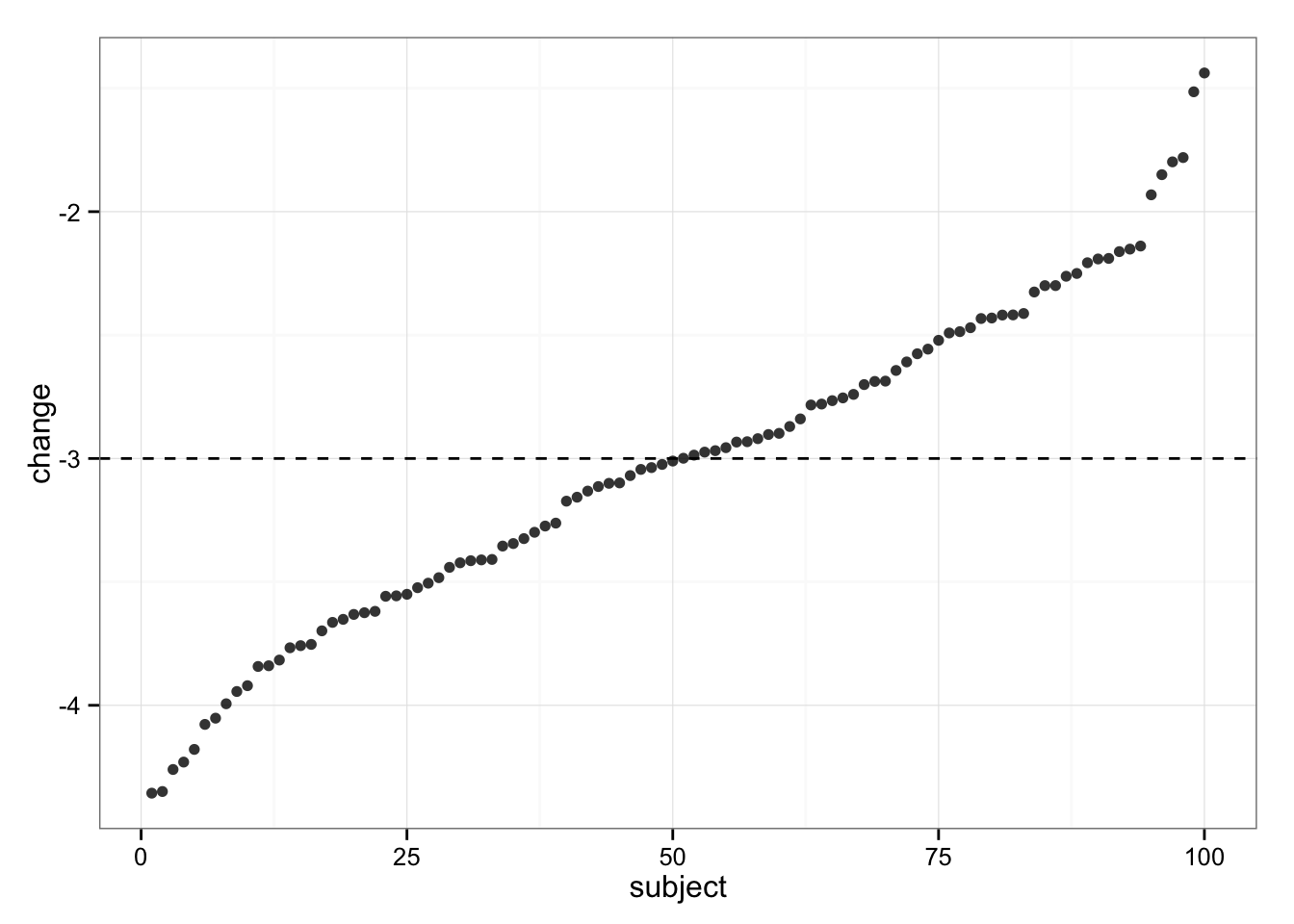
As can be seen, all subjects dropped weight, but some were in trivial zone (less than SWC, or 3kg). These individuals must be non-responders! But wait…
Since we simulated the data we KNOW that each individual experienced “real” change of -3kg (hence no “true” individual differences in response). So, our variability in change (response) is NOT the result of individual differences in response (responders vs. non-responders), but rather due typical variation in the measurement.
What if we plot confidence interval (CI) around each change? We know that typical variation is 0.5kg, hence the 95% CI would be approximately 2*TV.
limits <- data.frame(ymax = sort(change.intervention.measured.BW) - 2 * TV,
                     ymin = sort(change.intervention.measured.BW) + 2 * TV)

# Plot
gg <- ggplot(data.frame(change = sort(change.intervention.measured.BW),
                        subject = 1:100 ))
gg <- gg + geom_errorbar(data = limits, aes(ymin = ymin, ymax = ymax, x = 1:100), color = "grey")
gg <- gg + geom_point(aes(y = change, x = subject),
                    alpha = 0.8,
                    color = "black",
                    stat = "identity")
gg <- gg + theme_bw()
gg <- gg + geom_hline(yintercept=-3, linetype = 2)
gg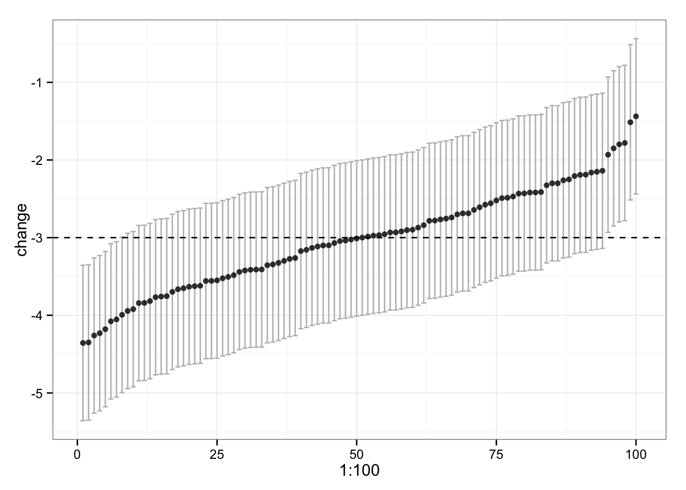
We can see that some of our subjects’ CI don’t touch the -3kg, which is “real” change. Why is that? Because of multiple comparison (correct me if I am wrong here). 95% will caught “real” change in 95 out of 100 times, so we have good number of comparisons to make this happen. Even the confidence intervals lie sometimes.
Let’s see what’s happening with Control group
change.control.measured.BW <- post.control.measured.BW - pre.control.measured.BW

# Plot
gg <- ggplot(data.frame(change = sort(change.control.measured.BW),
                        subject = 1:100 ))
gg <- gg + geom_point(aes(y = change, x = subject),
                    alpha = 0.8,
                    fill = "grey",
                    stat = "identity")
gg <- gg + theme_bw()
gg <- gg + geom_hline(yintercept=0, linetype = 2)
gg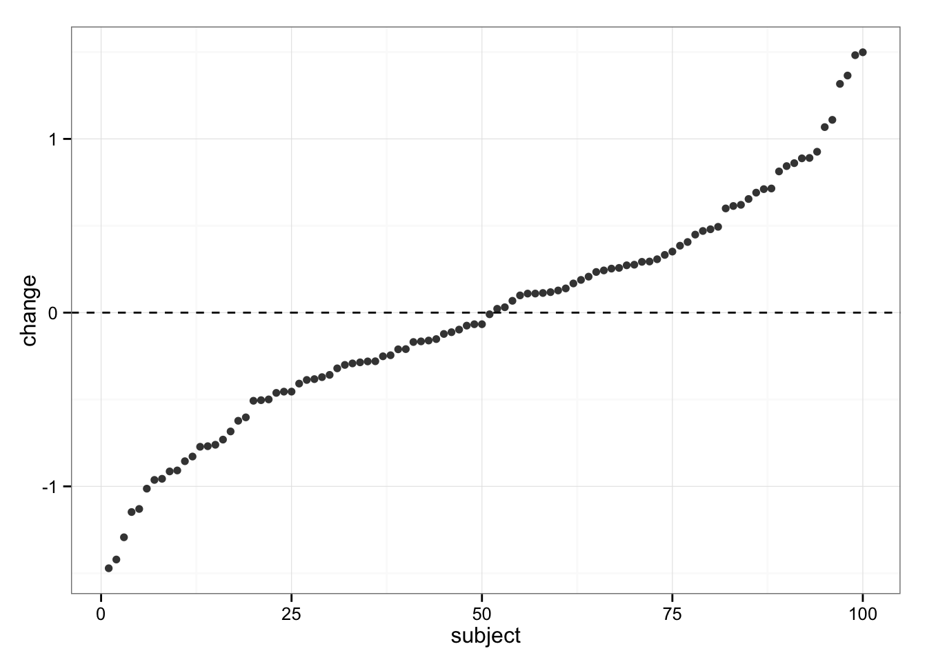
We can see same variability in responses, but we know the “real” change in Control group is 0 (zero).
The problem is then making confidence in stating that there are “real” individual differences in response and not “artefacts” based on typical variation and regression to the mean.
Solution?
Since this is simulation we know the “real” values, but in real life we never know them. So before we make any claims on who is responder and who is non-responder we need to take into account typical variations of the measurement. We need to know (or at least estimate) within-subject variation. Let me quote Atkinson and Batterham:
It is this random within-subjects variability that makes it appear that individuals have responded differently to an intervention, when in fact there might be clinically unimportant inter-individual differences in the true response to an intervention.
One way to quantify the “true” individual differences in response to an intervention would be to compare SDs of change scores to typical variation of the measurement. In our case, the SD of bodyweight change in the Intervention group is
sd(change.intervention.measured.BW)## [1] 0.661894And our typical variation is 0.5 kg. We also need to devide change SD with SQRT(2) to get typical variation
sd(change.intervention.measured.BW) / sqrt(2)## [1] 0.4680297We can see that they are very close. Same thing for Control group
sd(change.control.measured.BW) / sqrt(2)## [1] 0.4562379Since change SDs are comparable between Intervention and Control (and Typical Variation – or reliability study), we can conclude that individual variations are due random within-subject variations and NOT due variations in the intervention response.
Atkinson and Batterham suggested using SD of the Control group when reliability of the measurement is not available. The equation for calculating “real” individual response variability is as follows:
real.individual.response.SD <- sqrt(sd(change.intervention.measured.BW)^2 -
                                    sd(change.control.measured.BW)^2)
real.individual.response.SD
## [1] 0.1476399To assess if “real” individual differences are practically relevant we can use method suggested by Will Hopkins.
The baseline mean(SD) off all subjects pooled together is following:
pre.pooled <- rbind(pre.intervention.measured.BW,
                    pre.control.measured.BW)
mean(pre.pooled)
## [1] 100.933sd(pre.pooled)## [1] 15.00895So the baseline bodyweight is 101 (15) kg. The change in Intervention group is -3 (1) kg, and change in Control group is 0 (1) kg. The effect size (ES) of change (difference in mean change between Intervention and Control divided by baseline SD) is:
effect.size <- (mean(change.intervention.measured.BW) -mean(change.control.measured.BW)) / sd(pre.pooled)
effect.size
## [1] -0.2004912The effect size is -0.2, which is trivial change. We selected -3 kg since it is 0.2 * SD or SWC in the simulation. Hence this is correct estimate. We can create CI around this point-estimate to make inferences to the population via bootstrap (I hate formulas), but I will skip it this time.
Ok, so the main effect is trivial. What can we say about individual responses? We have already calculated SD of individual responses to training free of noise (within-subject variation), but let’s do it again.
real.individual.response.SD <- sqrt(sd(change.intervention.measured.BW)^2 -
                                    sd(change.control.measured.BW)^2)
real.individual.response.SD
## [1] 0.1476399So the estimated “real” SD of individual responses is 0.15 kg. How practically relevant is this value? Will Hopkins uses normalization of this SD by dividing it with baseline SD
norm.real.individual.response.SD <- real.individual.response.SD / sd(pre.pooled)
norm.real.individual.response.SD
## [1] 0.009836794So the normalized individual response SD is 0.01, which is basically 0 (zero). Hence we can conclude that the variation in the responses in Intervention group are purely due to the “noise” (SD = 0.15kg, ES = 0.01).
Conclusion
Before we tag anyone as responder and non-responder we need to take into account random within-subjects variation and SWC of a given measure/test.
Be very cautious when someone is trying to sell you the responder vs. non-responder story.


Responses