{LEVsim}: Theoretical Load-Exertion-Velocity Model – Part 4: Prescription and Monitoring

Previous Part:

{LEVsim}: Theoretical Load-Exertion-Velocity Model – Part 3

Prescribing load

In the previous parts, prescribed load that needs to be lifted was prescribed as an absolute weight (e.g., 130 \(kg\)). {LEVsim} allows to prescribe load to be lifted using (1) absolute load, (2) percent of \(L_0\), (3) percent of profile \(1RM\), (4) percent of visit \(1RM\), (5) and percent of prescription (or planning) \(1RM\). I will walk you through each of these in this section.

Using absolute load as a prescription is the simplest approach, and all other methods represents ways to calculate an absolute load (given some parameter to normalize the load using percentage). The problem with this approach is of course individualization – i.e., depending on individual profile, some athletes might find certain load too high or too low.

Here is an example. Imagine we have three athletes. All three athletes have \(V_0\) equal to 2 \(ms^{-1}\), \(v1RM\) equal to 0.25 \(ms^{-1}\), and 4% \(L_0 \; Rep \; Drop\) (see previous part for more information). We will not use any errors/noise in this example (i.e., for repetition velocity, nor for perceived RIR ratings). Where these three athletes differ is the \(L_0\) parameter, set to be equal to 150, 175, or 200 \(kg\) respectively. Calculated profile 1RMs are thus equal to 131, 153, and 131 \(kg\) respectively. Let us call these athletes “Weak Athlete”, “Average Athlete”, and “Strong Athlete”.

Now, imagine we prescribe one set of five (1x5) with 125 \(kg\) to these three athletes, given {LEVsim} model. I will continue using the arrow graph introduced in the previous installment since it provides neat visual summary. The refresher: the arrow graph indicated the load, eRIR of the last repetition, and the arrow represent first/best and or last/worst measured repetition velocity (if not indicated otherwise, it is best and last measured repetition velocity). The result can be seen in Figure 1.

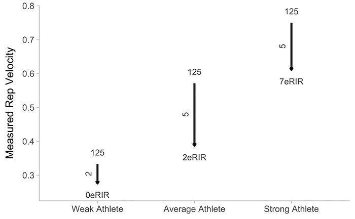
Figure 1: Three different athletes doing 1×5 with 125

As expected, given different \(L_0\), lifting same absolute load resulted in athletes demonstrating different lifting velocities, but more importantly, different exertion levels (i.e., expressed as eRIR; or true RIR in this case since there is no noise involved). “Weak Athlete” didn’t even manage to lift for 5 reps, and ended up doing 2 reps to failure.

How do we create more equal playing field (i.e., individualize) when profiles differ?

It is natural to suggest using \(L_0\) to prescribe load. Let us use 70% of \(L_0\) to prescribe training load to our three athletes. The result is depicted in Figure 2, but with extra two athletes, which are copies of the “Strong Athlete”: (1) “Strong Grinder”, which has all same parameter values, but the \(v1RM\) is much lower and equal to 0.1 \(ms^{-1}\), and (2) “Strong Explosive”, which has 20% higher \(V_0\) parameter.

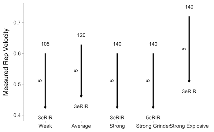
Figure 2: Five different athletes doing 1×5 with 70% of \(L_0\).

What can we conclude from Figure 2? For our first three athletes with different \(L_0\) parameter values, but every other parameter the same, using percentage of \(L_0\) yields same exertion reached (i.e., 3RIR). But for the “Strong Grinder” which has lower \(v1RM\), the exertion was lower (i.e., further away from failure; since he can bang more reps at certain % \(L_0\) due to lower \(v1RM\)). “Strong Explosive” athlete also reached same exertion level, but as expected, demonstrated higher starting and stopping velocity.

Next natural step is to use profile \(1RM\) to prescribe load. I will repeat the same experiment with the same athletes but will use 80% of profile \(1RM\). The results are depicted in Figure 3. This methods resulted in the same exertion (i.e., proximity to failure, expressed as RIR). This is because in our simulation all athletes have the same between-reps fatigue effect. Also note that the loads are rounded to the closes 2.5 \(kg\), since that is the realistic load we can lift in the gym due to plate limitations.

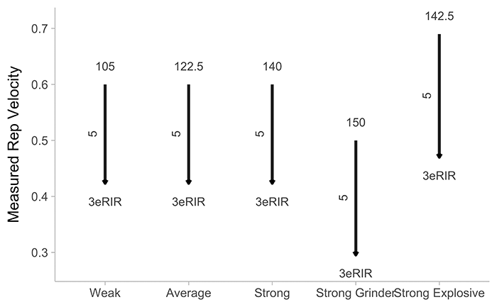
Figure 3: Five different athletes doing 1×5 with 80% of profile 1RM.

What is the problem with using profile \(1RM\) to prescribe? Well, since this is simulation, there is no problem at all. But in the real life we do not know the daily or visit \(1RM\). We need to estimate it. There are few methods to do so – for example, one might use warm-up sets and use either velocity or perceived exertion to estimate current \(1RM\). Or just test the \(1RM\) by using progressive loads. The problem with the former is error introduced by models used. If one uses velocity, to predict 1RM from submax sets, one needs to know individual and exercise specific \(v1RM\). The measuring device also needs to be precise enough. If one uses perceived exertion (i.e., RIR), then one must trust this perception. I have explained this method in the Create Custom Set and Rep Schemes With {STMr} course. The latter method of actually testing \(1RM\) is problematic since it takes time, and it takes energy from the athlete. Besides, who in the world would do that for all exercises done in the workout?