{LEVsim}: Theoretical Load-Exertion-Velocity Model – Part 3: RIR, Between-set, and Between-Visit Effects
Previous Part:
 {LEVsim}: Theoretical Load-Exertion-Velocity Model – Part 2
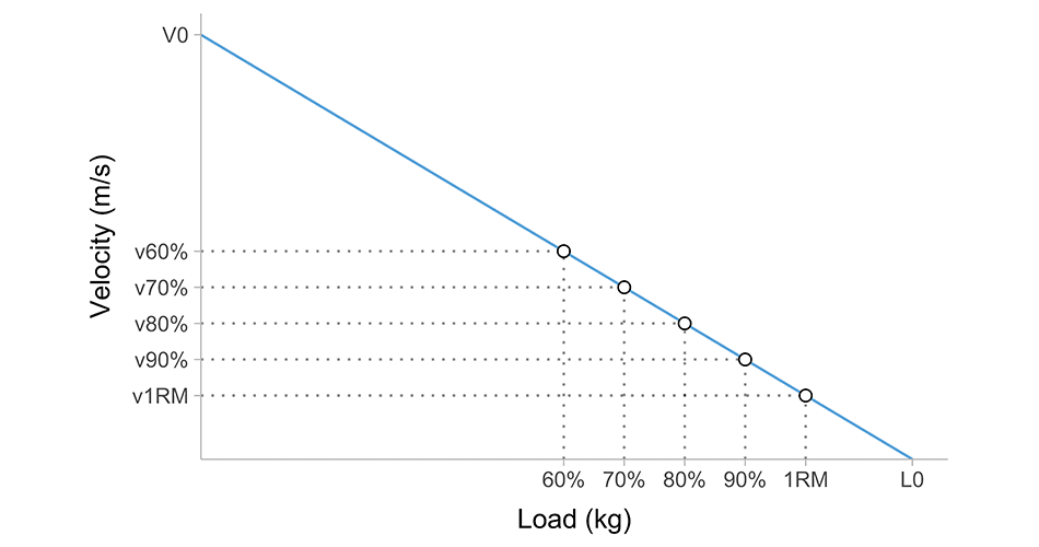
In the previous installment, we have covered (1) load-velocity profile (LVP) and parameters used to generate it (i.e., \(L_0\), \(V_0\) and \(v1RM\) with resulting profile \(1RM\)), (2) measurement error due to biological variation, instrumentation noise, repetition binning, and load rounding, and (3) within-set (i.e., between-reps) effects using \(Rep \; Drop\). These elements (i.e., layers) of the {LEVsim} model allow for simulation of the (1) relationship between load and velocity, (2) relationship between load and maximal number of reps, and (3) relationship between repetition velocity and proximity to failure phenomena we observe in the wild (i.e., Large or Real World).
In this installment we need to cover additional layers of the {LEVsim} model, namely the (1) subjective ratings of the set exertion using subjective, perceived, or estimated reps-in-reserve (eRIR or pRIR), (2) between-sets effects (i.e., fatigue between sets), and (3) between visits or between sessions effects (adaptation and/or fatigue between training).
Perceived (Estimated) Reps-In-Reserve
So far in the simulations involved in the previous installment all sets are taken to the failure. This allows us to calculate true rep-in-reserve (RIR) value for each individual rep. This is simply done by counting backwards from the failure point.
But in the real world, not all sets are taken to failure, of course. We can thus stop the sets before reaching failure. In real world, in that case we would not know the true RIRs of each individual rep (because we will not know where the point of failure is). But since this is generative formal model, in {LEVsim} we do know that, since all sets are simulated to failure and then capped if needed. In plain English, with {LEVsim} we do know each individual true RIR even if the set is not take to failure.
Let us use the following parameters for the simulation: \(V_0\) equal to 2 \(ms^{-1}\), \(L_0\) equal to 200 \(kg\), and \(v1RM\) is equal to 0.25 \(ms^{-1}\). Calculated \(1RM\) (i.e., expected 1RM based on LV profile) is in this case equal to 175 \(kg\). We are going to utilize 4% \(L_0 \; Rep \; Drop\) as our within-set fatigue parameter, since it was closest to the Epley’s model. We are going to use zero (i.e., nil) measurement error (i.e., biological variation and instrumentation error) in this case. Let us assume that this individual does single set to failure with 150 \(kg\) (approx. 86% 1RM).
Table 1 contains resulting individual rep RIRs and movement velocities. What is also included in the Table 1 are the individual rep \(V_0\) and \(L_0\), which change (only \(L_0\) decreased here since we utilized 4% \(L_0 \; Rep \; Drop\)) due to within-set fatigue effects, explained in the previous installment.
| set | load | rep | rep V0 | rep L0 | RIR | velocity |
|---|---|---|---|---|---|---|
| 1 | 150 | 1 | 2 | 200 | 4 | 0 |
| 1 | 150 | 2 | 2 | 194 | 3 | 0 |
| 1 | 150 | 3 | 2 | 188 | 2 | 0 |
| 1 | 150 | 4 | 2 | 182 | 1 | 0 |
| 1 | 150 | 5 | 2 | 176 | 0 | 0 |
Table 1: Sample set with 150 kg.
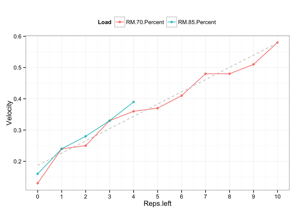
If we stop this set at rep 3 for example, we will be able to estimate true RIR of the last rep (Table 2). In real life we do not know this, so we need to rely to subjective ratings, or estimated RIR (eRIR). When set is taken to failure (i.e., 0RIR), the estimated and true RIR are equal (more about this in few paragraphs). With all other sub-max sets (i.e., sets not take to failure) there is some error involved, making these two differ.
| set | load | target reps | reps done | last rep RIR | best rep velocity | last rep velocity |
|---|---|---|---|---|---|---|
| 1 | 150 | 6 | 5 | 0 | 0.5 | 0.30 |
| 2 | 150 | 5 | 5 | 0 | 0.5 | 0.30 |
| 3 | 150 | 4 | 4 | 1 | 0.5 | 0.35 |
| 4 | 150 | 3 | 3 | 2 | 0.5 | 0.40 |
| 5 | 150 | 2 | 2 | 3 | 0.5 | 0.45 |
| 6 | 150 | 1 | 1 | 4 | 0.5 | 0.50 |
Table 2: Sample set with 150 kg using different tagret reps.
To formalize this relationship, {LEVsim} utilized (1) systematic and (2) random effects or errors, and both can be additive and multiplicative. Systematic effects are fixed – for example, if the true RIR of the last rep is equal to 3RIR (and we know this since we are using generative model), and the additive systematic effect is equal to +1, then the subject will always estimate it as 4 RIR. With multiplicative systematic effect, for example 40% (i.e., multiplicative factor equal to 1.4), then for true RIR of 3, athlete will estimate \(3 \times 1.4\) or 4.2RIR. Since we need to use counts, that will be equal to 4RIR. These systematic effects are depicted in Figure 1.
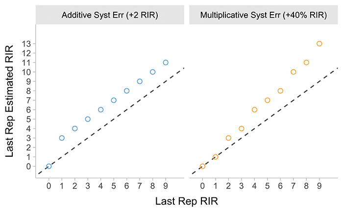
Figure 1: Systematic error effects on estimated last rep RIR.
Dashed line represent identity line, or the the perfect fit line on which all point would fall if there is no error.
Random effects are as the name suggest random, and follow the normal, Gaussian distribution, with standard deviation parameter sigma (\(\sigma\)) indicating value or strength of these random effects. For the additive random effect, the distribution mean is set to zero, while for the multiplicative random effect the distribution mean is set to one. Random effects on last repetition RIR are depicted in Figure 2.
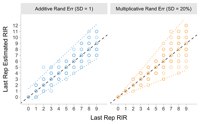
Figure 2: Random error effects on estimated last rep RIR. Dashed line represent identity line,
or the the perfect fit line on which all point would fall if there is no error. Dotted lines represent 0.01 and 0.99 quantile regression. Simulation repeated 20 times
Please note that we are using the true RIR of the last repetition in the set to calculate estimated last rep eRIR. All other eRIRs for other preceding reps are simply increments of the last rep eRIR. Also note that eRIR cannot be negative number – thus if the calculated eRIR is below zero, it will be set to zero.
If you look at Figure 1 and Figure 2 you will notice that if true RIR is equal to zero, then the eRIR is also equal to zero. That means that the aforementioned errors are not applied in this case. This can be debated of course. If athlete performs last rep (i.e., 0RIR) and then tries another one, but fails, then the athlete will truly know that this is 0RIR and will align his or her perception and rate this as 0eRIR. This is the rationale behind the aforementioned feature. If the athlete performs the last rep (i.e., 0RIR), but in this case doesn’t try another one, then he or she might have biased estimate of RIR. In plain English, athlete actually reached 0RIR exertion, but thinks he has one more rep left in the tank. He believes that because he didn’t attempt another rep. Both of these features are implemented in {LEVsim} and an example is depicted in Figure 3.
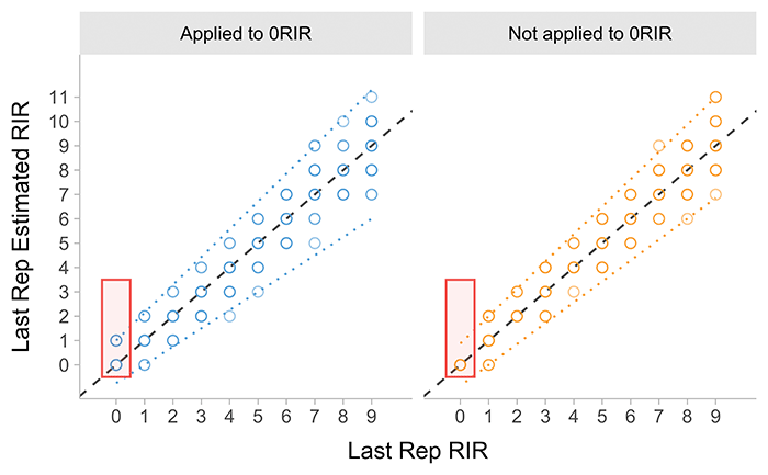
Figure 3: Difference when error effects are applied or not to 0RIR. Dashed line represent identity line,
or the the perfect fit line on which all point would fall if there is no error. Dotted lines represent 0.01 and 0.99 quantile regression. Simulation repeated 20 times
Also note that in Figure 3 (and all other preceding figures), athlete can have higher or lower estimated RIR compared to the true RIR. For example, when there is 1RIR, athlete might think there are 2RIR (over-confident), or he is she might believe there are no reps left in the tank (0RIR; or under-confident). In the latter example, if the athlete thinks there are zero reps left in the tank, but when forced to lift one more rep, he or she will find out that there are more reps left in the tank. The problem here is with the term forced that I have used. I think there are two components to this – one is the normal attempt, that yields more reps, and the second is facilitated attempt when someone else yells at you, increasing your intent, and might have the effect on the \(L_0\) and \(V_0\) parameters (given this theoretical model). The phenomena of these facilitated reps is not implemented in the {LEVsim}, but can be emulated with the random errors involved in the estimated RIR. I have expanded a bit more on this problem in Problem With (Perceived) Reps-In-Reserve article. Unfortunately, implementing all phenomena we observe in the Large World will beat the purpose of a simple model by making it too complex to utilize and understand. What is important is to keep in mind the distinction between the Large World and the Small World implementation, i.e., the model.


Responses