Force-Velocity Profiling in Resisted Sprinting – Part 1

The Latest Features of the {shorts} Package

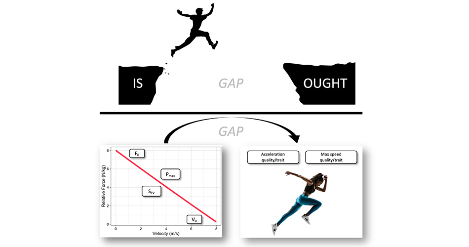
Force-Velocity Profile

Although you might already be familiar with my opinion regarding the Force-Velocity Profiling (FVP) in sprinting, I will review the basic concept and provide some novel developments in the {shorts} package, particularly for doing FVP for resisted sprinting. To install {shorts} package use the following code:

# Install from CRAN
install.packages("shorts")

# Or the development version from GitHub
# install.packages("remotes")
remotes::install_github("mladenjovanovic/shorts")

I will provide the R code for everything, just make sure to click the “Show the code” which is located over the code boxes.

Let us imagine we have an athlete with maximal-sprinting speed (\(MSS\)) of 9 \(ms^{-1}\) and maximal-acceleration (\(MAC\)) of 7 \(ms^{-2}\). These two parameters represent mathematical model of the short sprint performance, which is titled Acceleration-Velocity Profile (AVP). Simply, the AVP is a neat and mathematically elegant way to summarize, describe, and aggregate overall short sprint performance (e.g., < 6 \(sec\); or sprints which do not involve deceleration). As such, AVP represents a Small World model, or a map of the much more complex territory, but it is indeed very useful, as long as we are aware it is a map. Anyhow, we can estimate the AVP from various sources of performance data (with more or less issues; for example the effect of the flying start – see Jovanović (2023), as well recent article series), but here we are going to assume it as true. What I mean by this, is that we are going to generate sprint performance data using aforementioned \(MSS\) and \(MAC\) parameter values.

Additionally, we are going to assume that this athlete weights 90 \(kg\) and has height of 185 \(cm\). The conditions of the sprint involve no wind, 25 \(C^\circ\) temperature, and 760 \(torr\) air pressure. These are used to calculate wind resistance.

Figure 1 and Figure 2 depict horizontal sprint velocity (given the mathematical model with known parameters) across time and distance.

# Load packages
library(tidyverse)
library(shorts)
library(directlabels)
library(ggdist)

# Color set
color_transparent <- "transparent"
color_white <- "#FFFFFF"
color_black <- "#000000"
color_blue <- "#5DA5DA"
color_red <- "#F15854"
color_grey <- "#4D4D4D"
color_green <- "#60BD68"
color_orange <- "#FAA43A"
color_pink <- "#F17CB0"
color_purple <- "#B276B2"
color_yellow <- "#DECF3F"

# Parameters
MSS <- 9
MAC <- 7
bodymass <- 90
bodyheight <- 1.85

kinematics <- predict_kinematics(
  MSS = MSS,
  MAC = MAC,
  bodymass = bodymass,
  bodyheight = bodyheight,
  frequency = 20)

time_to_95 <- find_velocity_critical_time(MSS, MAC, 0.95)

kinematics %>%
  ggplot(aes(x = time, y = velocity)) +
  geom_hline(yintercept = 0, linetype = "dotted", alpha = 0.3) +
  geom_vline(xintercept = 0, linetype = "dotted", alpha = 0.3) +
  geom_point(shape = 21) +
  geom_hline(yintercept = MSS * 0.95, linetype = "solid", color = color_red) +
  geom_vline(xintercept = time_to_95, linetype = "solid", color = color_red) +
  xlab("Time (s)") +
  ylab("Velocity (m/s)")

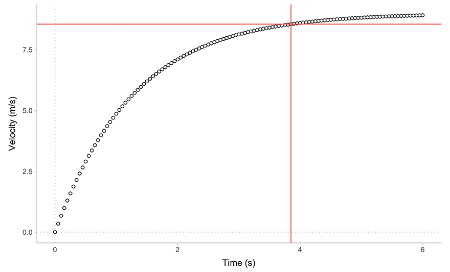
Figure 1: Sample time-velocity trace of a short sprint with known \(MSS\) and \(MAC\) parameters. Dotted line represent time it takes to reach 95% of MSS

dist_to_95 <- find_velocity_critical_distance(MSS, MAC, 0.95)

kinematics %>%
  ggplot(aes(x = distance, y = velocity)) +
  geom_hline(yintercept = 0, linetype = "dotted", alpha = 0.3) +
  geom_vline(xintercept = 0, linetype = "dotted", alpha = 0.3) +
  geom_point(shape = 21) +
  geom_hline(yintercept = MSS * 0.95, linetype = "solid", color = color_red) +
  geom_vline(xintercept = dist_to_95, linetype = "solid", color = color_red) +
  xlab("Distance (m)") +
  ylab("Velocity (m/s)")

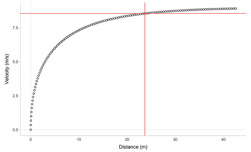
Figure 2: Sample distance-velocity trace of a short sprint with known \(MSS\) and \(MAC\) parameters. Dotted line represent distance it takes to reach 95% of MSS

Figure 3 depicts acceleration across distance. Given this model, the highest acceleration (i.e., \(MAC\)) happens at \(t=0s\) and reaches zero when the velocity reaches maximum (i.e., \(MSS\)). This is a strong assumption, since in some standing start cases, the initial acceleration is not maximal, since there is some roll over (see “Issues at the start” in this installment).

kinematics %>%
  ggplot(aes(x = distance, y = acceleration)) +
  geom_hline(yintercept = 0, linetype = "dotted", alpha = 0.3) +
  geom_vline(xintercept = 0, linetype = "dotted", alpha = 0.3) +
  geom_point(shape = 21) +
  xlab("Distance (m)") +
  ylab("Acceleration (m/s/s)")

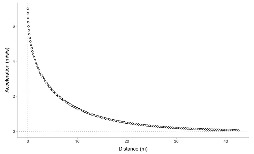
Figure 3: Sample distance-acceleration trace of a short sprint with known \(MSS\) and \(MAC\) parameters.

The neat thing about the AVP is that if we plot the relationship of the velocity against acceleration, we will get Figure 4. Interestingly, it is linear, hence the name profile, which we can summaries with two points, or parameters: (1) \(MSS\) is the velocity where acceleration is zero, or where our line/profile crosses the x-axis, and (2) \(MAC\) is the acceleration where velocity is zero, or where our line/profile crosses the y-axis. Thus, the \(MSS\) and \(MAC\) are just another way to represent a line, which is usually represented with the intercept (equal to \(MAC\)) and slope (equal to \(-\frac{MAC}{MSS}\)).

kinematics %>%
  ggplot(aes(x = velocity, y = acceleration)) +
  geom_hline(yintercept = 0, linetype = "dotted", alpha = 0.3) +
  geom_vline(xintercept = 0, linetype = "dotted", alpha = 0.3) +
  geom_point(shape = 21) +
  ylab("Acceleration (m)") +
  xlab("Velocity (m/s)") +
  annotate("label", x = 0, y = MAC, label = "MAC") +
  annotate("label", y = 0, x = MSS, label = "MSS")

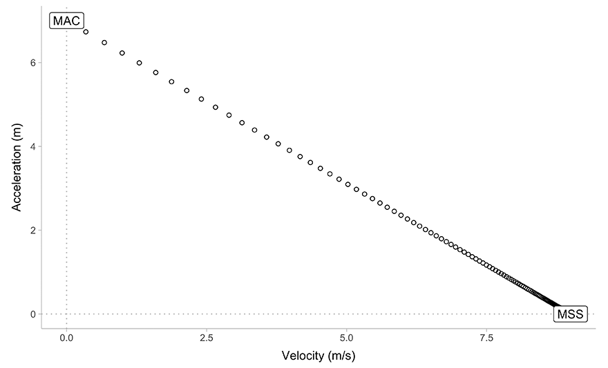
Figure 4: Sample velocity-acceleration trace of a short sprint with known \(MSS\) and \(MAC\) parameters.

Since we know the AVP and we have the information to estimate the air resistance, we can also calculate the instantaneous horizontal force (Figure 5).

kinematics %>%
  ggplot(aes(x = distance, y = horizontal_force)) +
  geom_hline(yintercept = 0, linetype = "dotted", alpha = 0.3) +
  geom_vline(xintercept = 0, linetype = "dotted", alpha = 0.3) +
  geom_point(shape = 21) +
  ylab("Force (N)") +
  xlab("Distance (m)")

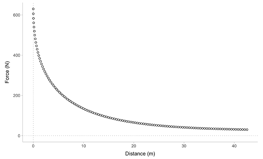
Figure 5: Sample distance-horizontal force trace of a short sprint with known \(MSS\) and \(MAC\) parameters, as well as the estimated air resistance

What you can notice in Figure 5 as opposed to the Figure 3 is that force never reaches zero, which is of course due to air resistance (Figure 6).

kinematics %>%
  ggplot(aes(x = distance, y = air_resistance)) +
  geom_hline(yintercept = 0, linetype = "dotted", alpha = 0.3) +
  geom_vline(xintercept = 0, linetype = "dotted", alpha = 0.3) +
  geom_point(shape = 21) +
  ylab("Air resistance (N)") +
  xlab("Distance (m)")

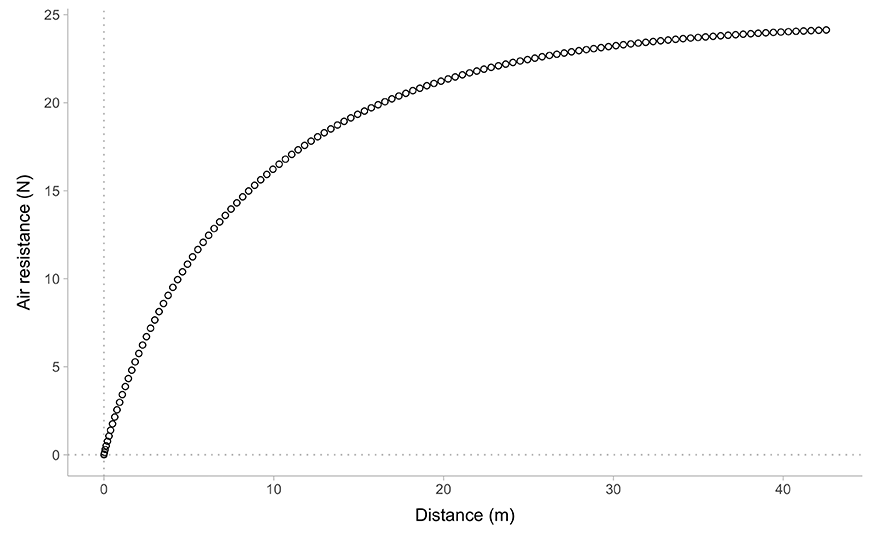
Figure 6: Sample distance-air resistance trace of a short sprint with known \(MSS\) and \(MAC\) parameters

One way we can plot the acceleration versus horizontal force is to normalize the force by dividing by bodyweight (Figure 7). The difference between the two, is that acceleration is net propulsive horizontal force, while horizontal force involves both net propulsive force as well as the air resistance.

kinematics %>%
  ggplot(aes(x = distance)) +
  geom_hline(yintercept = 0, linetype = "dotted", alpha = 0.3) +
  geom_vline(xintercept = 0, linetype = "dotted", alpha = 0.3) +
  geom_point(aes(y = acceleration, color = "acceleration"), shape = 21) +
  geom_point(aes(y = horizontal_force_relative, color = "relative horizontalforce"), shape = 22) +
  ylab("Relative force (N/kg)") +
  xlab("Distance (m)") +
  theme(legend.position = "right", legend.title = element_blank()) +
  scale_color_manual(values = c("acceleration" = color_blue, "relative horizontalforce" = color_orange))

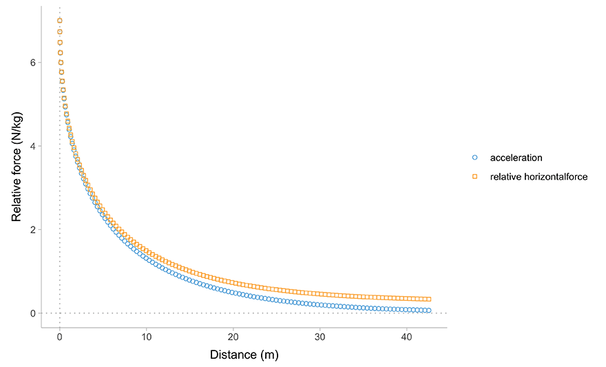
Figure 7: Difference between acceleration and relative force of a short sprint with known \(MSS\) and \(MAC\) parameters. Red dots indicate relative force

Rather than using acceleration and velocity to get the AVP (Figure 4), we can plot force, or relative force against velocity to get Force-Velocity Profile (FVP), as depicted in Figure 8.

FVP <- create_FVP(
  MSS = MSS,
  MAC = MAC,
  bodymass = bodymass,
  bodyheight = bodyheight
)

F0 <- FVP$F0
V0 <- FVP$V0

kinematics %>%
  ggplot(aes(y = horizontal_force_relative, x = velocity)) +
  geom_point(shape = 21) +
  geom_abline(intercept = FVP$F0_rel, slope = -(FVP$F0_rel/FVP$V0), color = color_red) +
  geom_hline(yintercept = 0, linetype = "dotted", alpha = 0.3) +
  geom_vline(xintercept = 0, linetype = "dotted", alpha = 0.3) +
  #scale_y_continuous(expand = c(0, 0), limits = c(0,  FVP$F0_rel)) +
  #scale_x_continuous(expand = c(0, 0), limits = c(0, FVP$V0)) +
  ggtitle(
    label = "Force-Velocity Profile",
    subtitle = paste0(
      "MSS = ", round(MSS, 2), " m/s; MAC = ", round(MAC, 2), " m/s/s\n",
      "V0 = ", round(FVP$V0, 2), " m/s; F0_rel = ", round(FVP$F0_rel, 2), " N/kg; F0 = ", round(FVP$F0, 2), " N")
  ) +
  ylab("Relative Horizontal Force (N/kg)") +
  xlab("Velocity (m/s)") +
  xlim(NA, 10) +
  annotate("label", x = 0, y = FVP$F0_rel, label = "F0 rel") +
  annotate("label", y = 0, x = FVP$V0, label = "V0")

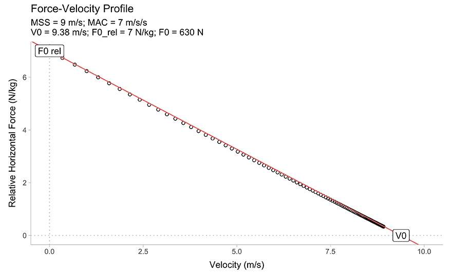
Figure 8: Sample velocity-relative horizontal force trace of a short sprint with known \(MSS\) and \(MAC\) parameters with estimated air resistance. Red line represent the FVP

As you can notice in Figure 8, the relationship between horizontal force and velocity is not exactly linear, but it is often represented with a simple linear model. Same as with the AVP, this linear model have intercept and slope parameters, which is often more intuitively represented by two extreme points, \(F_0\) (or relative \(F_0\)) and \(V_0\). These two parameters can be estimated via (1) simulation or quantitatively, and (2) analytically by solving a simple equation (i.e., by finding velocity when force is zero for \(V_0\), and force when velocity is zero for \(F_0\)). This is simply imagined if you extend the line and find where it crosses the x- and y-axes.

{shorts} package provides a function shorts::create_FVP() which estimates the \(F_0\) and \(V_0\) parameters using the analytic method. The solution is depicted as red line in Figure 8.

Once we have the force and velocity, we can calculate horizontal power (Figure 9). With AVP and FVP, there are three maximum power estimates.

• \(PMAX\), which is net relative propulsive power is equal to \(MSS \times MAC \times \frac{1}{4}\). This is maximum relative power at propelling the body, without the air resistance. Estimated \(PMAX\) is equal to 15.75 \(W/kg\)
• Pmax, is calculated similarly as \(PMAX\), but it takes the FVP parameters into account, and thus includes air resistance into calculus. It is calculates as \(F_0 \times V_0 \times \frac{1}{4}\). If we divide this by bodyweight, we will get the relative Pmax. This equation is just a simple proxy to calculating peak power, assuming the linear relationship between force and velocity, but as we have seen in Figure 8, they are not exactly linear (but very close to). Estimated Pmax is equal to 16.42 \(W/kg\)
• PeakPower is THE peak manifested horizontal power, which needs to be estimated quantitatively and it is equal to 16.07 \(W/kg\). As you can notice, Pmax and PeakPower are quite similar, but not the same.

There are other ways to calculate power, for example, average power over some distance and using velocity of a single point (or average) and multiplying it with resistance. But we will deal with those in a bit.

peakPower <- find_peak_power_distance(
  MSS = MSS,
  MAC = MAC,
  bodymass = bodymass,
  bodyheight = bodyheight
)

kinematics %>%
  ggplot(aes(x = distance, y = power_relative)) +
  geom_point(shape = 21) +
  geom_hline(yintercept = FVP$Pmax_rel, linetype = "dotted", color = color_blue) +
  geom_hline(yintercept = peakPower$peak_power / bodymass, linetype = "dotted", color = color_red) +
  geom_vline(xintercept = peakPower$distance, linetype = "dotted", color = color_red) +
  geom_hline(yintercept = MSS * MAC / 4, linetype = "dotted", color = color_grey) +
  annotate("label", x = 35, y = FVP$Pmax_rel, label = "Pmax") +
  annotate("label", x = 10, y = MSS * MAC / 4, label = "PMAX") +
  annotate("label", x = 25, y = peakPower$peak_power / bodymass, label = "PeakPower") +
  ylab("Relative Power (W/kg)") +
  xlab("Distance (m)")

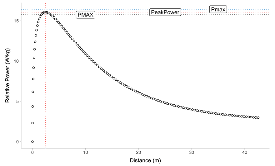
Figure 9: Sample distance-horizontal power trace of a short sprint with known \(MSS\) and \(MAC\) parameters. Horizontal lines represent three types of max power: (1) \(PMAX\) – grey, (2) Pmax – blue, and (3) PeakPower – red.

Adding load (i.e., resistance)

So far we have estimated FVP under unloaded sprint conditions. But we can add load to the athlete, of course. There are few ways to load the sprint: