Effect of Typical Variation of a Test on Confidence Interval

Confidence intervals gives us the range of a given statistic when generalizing from a sample to a population. The simplest example could be mean of a sample (e.g. average height) – what we are interested in are the generalizations (or inferences) from this sample to a population (e.g. average height in population). Due the sampling error we are not very confident in point-estimates and we are interested in a range os such a statistic in a population.

What I am interested is how the typical variation of a given test (e.g. vertical jump height) affects the confidence interval of a statistic. The lower the reliability of a test, the lower we are certain of a true single-subject score or a sample mean, and hence less certain of a the range in the population.

This article is my “workbook” and by no means represents any significant work or valid approach. It is just me “thinking out loud”. By all means, I eager statiscians and researchers out there to double check what I’ve done here and provide some guidelines.

Anyway, since I like algorythms more than math, I actually prefer the modern statistical methods such as bootstrap. Bootstrap is very simple idea and yet very powerful. Bootstap basically resamples the sample numerous times and use that to predict the population confidence interval.

For this simple workbook, I will use bodyweight estimate. Assume we tested 50 athletes (N = 50, mean = 85, SD = 10), and we are interested in making generalizations to the athletic population (or a subset from which we randomly sampled those athletes) and figure out what would be the likely average weight.

set.seed(1) # Set the random number generator seed to 1 (or any other number) so you can reproduce the same results
number.of.athletes <- 50
sample.weight <- rnorm(n=number.of.athletes, mean=85, sd=10)

hist(sample.weight)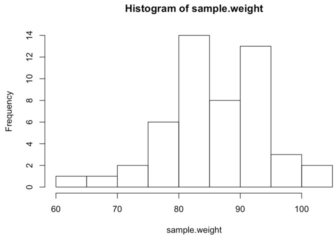

But without taking the scale “unreliability” into account, we are interested in making the generalizations to the population. Using sample mean, we can easily calculate standard error (I have no clue why it is called “standard error” – I preffer to call is “sampling error”) and provide confidence interval of the sample mean (using t-test). But this time, I will code my own bootstrap algorithm and compare.

# Perform a simple t-test to get the sample mean and confidence interval
t.test(sample.weight)

## 
##  One Sample t-test
## 
## data:  sample.weight
## t = 73.1475, df = 49, p-value < 2.2e-16
## alternative hypothesis: true mean is not equal to 0
## 95 percent confidence interval:
##  83.64169 88.36728
## sample estimates:
## mean of x 
##  86.00448

# Pull out confidence interval by using linear regression approach
confint(lm(sample.weight ~ 1))

##                2.5 %   97.5 %
## (Intercept) 83.64169 88.36728

# Now let's code bootstrap approach
resampling <- 20000

bootstrap.mean <- rep(0, resampling) # Generate a vector with 20000 elements

for ( i in 1:resampling)
    {
    # Create a sample from a sample with same number of subjects and replacements
    bootstrap.sample <- sample(sample.weight, size = number.of.athletes, replace = TRUE)
    
    # Calculate the mean of the bootstrap sample and save it in the vector
    bootstrap.mean[i] <- mean(bootstrap.sample)
    }

# Here is the histogram of our bootstraped sample mean
hist(bootstrap.mean)

# And calculate the confidence interval
quantile(bootstrap.mean, c(0.025, 0.975))

##     2.5%    97.5% 
## 83.68861 88.20193

If you compare the 95% confidence interval between t-test and bootstrap you can quickly see that they are very close.

Now, let’s add typical error (unrealiability of the scale) in every observation (remember, SD = 1kg) and see how will that affect our confidence interval

bootstrap.mean.with.TE <- rep(0, resampling) # Generate a vector with 20000 elements

for ( i in 1:resampling)
    {
    # Create a sample from a sample with same number of subjects and replacements
    bootstrap.sample.with.TE <- sample(sample.weight, size = number.of.athletes, replace = TRUE) +
                                rnorm(n = number.of.athletes, mean = 0, sd = 1)
    
    # Calculate the mean of the bootstrap sample and save it in the vector
    bootstrap.mean.with.TE[i] <- mean(bootstrap.sample.with.TE)
    }

# Here is the histogram of our bootstraped sample mean
hist(bootstrap.mean.with.TE)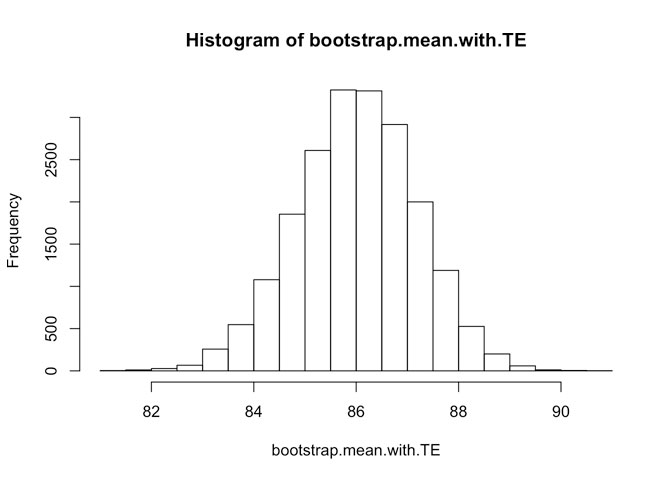

# And calculate the confidence interval
quantile(bootstrap.mean.with.TE, c(0.025, 0.975))

##     2.5%    97.5% 
## 83.67143 88.22728

This is slightly wider interval. What we can do is to use robust Smirnov-Kolmogorov test to estimate are these two results (i.e. without and with typical error) “drawn” from the same population (i.e. population of same variance).

ks.test(bootstrap.mean, bootstrap.mean.with.TE)

## 
##  Two-sample Kolmogorov-Smirnov test
## 
## data:  bootstrap.mean and bootstrap.mean.with.TE
## D = 0.0072, p-value = 0.6693
## alternative hypothesis: two-sided

Although wider, the difference is not statisticaly significant (where the null hypothesis is that both samples come from same population).

Let’s make a simple simulation. Let’s calculate boostrapped confidence interval of our measure, but vary the typical error of the scale, from 0 to 5 to see how does confidence interval changes, along with Smirnov-Kolgomorov test

typical.errors <- seq(0, 5, length.out = 20)
bootstrap.mean.with.TE <- rep(0, resampling) # Generate a vector with 20000 elements
results.table <- data.frame(TE = rep(0, 20), lowCL = rep(0, 20),
                            highCL = rep(0, 20), SE = rep(0, 20), 
                            p.value = rep(0, 20))

for (TE in 1:20)
    {
    for ( i in 1:resampling)
        {
        # Create a sample from a sample with same number of subjects and replacements
        bootstrap.sample.with.TE <- sample(sample.weight, size = number.of.athletes, replace = TRUE) +
                                    rnorm(n = number.of.athletes, mean = 0, sd = typical.errors[TE])
    
        # Calculate the mean of the bootstrap sample and save it in the vector
        bootstrap.mean.with.TE[i] <- mean(bootstrap.sample.with.TE)
        }
    results.table$TE[TE] <- typical.errors[TE]
    results.table$lowCL[TE] <- quantile(bootstrap.mean.with.TE, 0.025)
    results.table$highCL[TE] <- quantile(bootstrap.mean.with.TE, 0.975)
    results.table$p.value[TE] <- ks.test(bootstrap.mean, bootstrap.mean.with.TE)$p.value
    results.table$SE[TE] <- sd(bootstrap.mean.with.TE)
    }

round(results.table, 2)

##      TE lowCL highCL   SE p.value
## 1  0.00 83.71  88.24 1.16    0.78
## 2  0.26 83.72  88.23 1.15    0.41
## 3  0.53 83.65  88.23 1.16    0.35
## 4  0.79 83.63  88.26 1.17    0.96
## 5  1.05 83.65  88.25 1.17    0.92
## 6  1.32 83.70  88.25 1.17    0.25
## 7  1.58 83.65  88.25 1.18    0.22
## 8  1.84 83.64  88.27 1.19    0.63
## 9  2.11 83.58  88.28 1.20    0.10
## 10 2.37 83.58  88.32 1.21    0.06
## 11 2.63 83.56  88.35 1.22    0.00
## 12 2.89 83.51  88.38 1.24    0.01
## 13 3.16 83.56  88.40 1.24    0.00
## 14 3.42 83.47  88.43 1.27    0.00
## 15 3.68 83.48  88.42 1.26    0.00
## 16 3.95 83.47  88.48 1.28    0.00
## 17 4.21 83.38  88.52 1.31    0.00
## 18 4.47 83.36  88.56 1.33    0.00
## 19 4.74 83.36  88.61 1.35    0.00
## 20 5.00 83.32  88.64 1.35    0.00

As can bee seen from the table, the reliability of the scale affects the confidence interval of the estimate (i.e. average bodyweight). It takes typical error bigger than 2kg (SD=2kg) for the confidence interval to be (statistically) significantly different from the confidence interval with perfect reliability.

I hope I haven’t done any major errors in my code and reasoning and hopefuly managed to “integrate” test reliability into confidence interval using bootstrap approach.