{LEVsim}: Theoretical Load-Exertion-Velocity Model – Part 2: LEVsim Model

Previous Part:

{LEVsim}: Theoretical Load-Exertion-Velocity Model – Part 1

Why we need formal computational theory?

I have introduced the very robust phenomena of resistance training: (1) trade-off between load and velocity, (2) trade-off between load and maximal number of reps, and (3) trade-off between repetition velocity and proximity to failure. Research on resistance training in general, and velocity-based training (VBT) in particular represents tremendous effort by the researchers in finding statistical effects in the collected data. Unfortunately, these results in conflations of the theoretical and statistical models (Fried 2020b). These models say very little about the processes that actually generated the data (DGP; data generating process) (P. E. Smaldino 2017). What is lacking are the formal theoretical and computational models, that transparently provide assumption, provide testable predictions, allows to simulate data under a theory, and enables the comparison of such theory-implied and simulated data with actual data (Guest and Martin 2021; Muthukrishna and Henrich 2019; P. E. Smaldino 2017; Borsboom et al. 2020; Fried 2020a, 2020b; P. Smaldino 2019).

The theoretical model I am about to present in this article series represent computational theoretical model (Guest and Martin 2021) that formalizes the assumptions of the underlying DGP, theorized to produce the aforementioned resistance training phenomena. Simulation of the model generated data allows for exploration and understanding of the effects of model parameters on the observed data. Finally, theoretical computational model allows for estimation of the prescription error, since we can compare the true values (i.e., generated values) with different prescription approaches. In addition, theoretical model can be a fruitful generator of the new hypotheses and can thus drive research attempts.

I have named this generative model LEVsim, or Load-Exertion-Velocity simulation model. There are multiple layers of this model, and in this article series I will explain each of them.

This model is implemented in the {LEVsim} R package. You can install the development version from GitHub with:

# install.packages("devtools")
devtools::install_github("mladenjovanovic/LEVsim")

require(LEVsim)

Load-Velocity Profile

The trade-off relationship between load and velocity can be formalized with a simple l inear relationship, forming individual’s load-velocity profile (LVP) (Figure 1). LVP is characterized with two parameters: \(L_0\) and \(V_0\) . These two parameters can be interpreted using realist ontology, or using instrumentalist ontology (Borsboom 2008, 2009; Borsboom, Mellenbergh, and van Heerden 2003; Yarkoni 2020; Fried 2020a, 2020b).

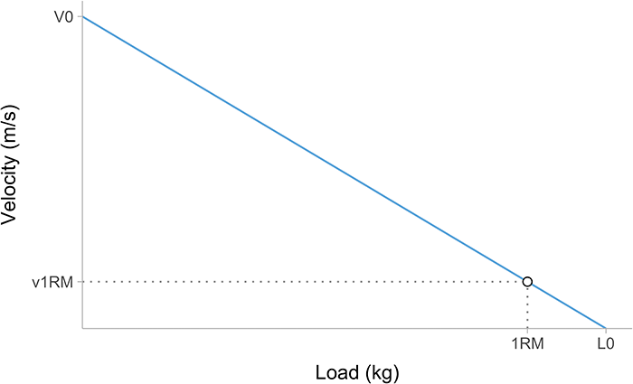
Figure 1: Load-Velocity Profile. In addition to the \(L_0\) and \(V_0\) parameters, two additional parameters are \(1RM\) and \(v1RM\). Please refer to the main text for explanation.

From a realist perspective, \(L_0\) represents maximal load that can be lifted in isometric conditions (i.e., when velocity equals zero), while \(V_0\) represents hypothetical maximal lifting velocity that can be achieved when there is no load (i.e., load is equal to zero).

From instrumentalist perspective, \(L_0\) and \(V_0\) represent just a different, and probably more intuitive, approach to describe a line. The equation for a straight line consists of \(intercept\) and \(slope\) parameters (Equation 1).

\[
y = intercept + slope \times x
\tag{1}\]

Equation 1 can be rewritten in the form of Equation 2.

\[
velocity = V_0 + -\frac{V_0}{L_0}\times load
\tag{2}\]

In Equation 2 form, \(intercept\) is equal to \(V_0\) and line \(slope\) is equal to \(-\frac{V_0}{L_0}\). In the case where velocity is the predictor, the Equation 2 get’s the form of Equation 3.

\[
load = L_0 + -\frac{L_0}{V_0}\times velocity
\tag{3}\]

In this theoretical model, \(L_0\) and \(V_0\) represent one of the key parameters of the DGP, and thus can have realist interpretation (i.e., they represent causal construct responsible for the model behavior and manifested performance).

One-repetition maximum and minimum velocity threshold

In addition to the LVP, two additional parameters are \(1RM\) and \(v1RM\) (Figure 1). One-repetition-maximum, or \(1RM\), represent maximal load that can be lifted with predefined technique (which includes, but it is not limited to, posture, range-of-movement, defined pauses and lifting tempo). Velocity associated with \(1RM\) attempt is termed velocity-at-one-repetition-maximum, or \(v1RM\), and according to the evidence so far, it seems to be rather stable across training intervention, and specific to the individual and exercise (Weakley et al. 2020).

In {LEVsim} model, \(v1RM\), in addition to \(L_0\) and \(V_0\), represents one of the key DGP parameters, while the \(1RM\) itself, represents the highest load that can be lifted given the \(v1RM\), \(L_0\), and \(V_0\) parameter values. In plain English, we set \(v1RM\), \(L_0\), and \(V_0\) parameter values, and calculate \(1RM\) as theoretical estimate, given this theoretical model parameter values. \(1RM\) is simply estimated by plugging the \(v1RM\), \(L_0\), and \(V_0\) values in Equation 3, giving Equation 4.

\[
1RM = L_0 + -\frac{L_0}{V_0}\times v1RM
\tag{4}\]

Velocity at \(1RM\) (i.e., \(v1RM\)), according to the current theoretical model, is also associated with the velocity of the last successfully performed repetition with sub-maximal load lifted to failure (e.g., 80% 1RM for 6 reps, where 7th rep was unable to be lifted with predefined technique). \(v1RM\) can also be termed minimum-velocity threshold (MVT) (Jovanović and Flanagan 2014), or velocity-at-zero-reps-in-reserve (v0RIR). This concept is further elaborated in later sections, but you can also check the previous installment of this article series.

Contemporary resistance training prescription, i.e. percent-based approach (PBT) (Jovanović 2020a), prescribes training loads using percent of \(1RM\), or relative loads (i.e., 65% \(1RM\), 90% \(1RM\)). Load-Velocity profile can thus also be expressed using relative loads, rather than absolute loads. This can be achieved by either using \(L_0\) or \(1RM\) (which is more common).

Under the assumptions of the current formal model, prescribing training loads using velocity associated with a particular %\(1RM\) (i.e., v65% \(1RM\), v90% \(1RM\)) (Figure 2), instead of using \(1RM\), is believed to be more robust to visit-to-visit fluctuations and chronic changes in \(1RM\), and thus represents improved approach in individualizing training load prescription. This hypothesis should be tested using simulation or using observed data and I will do that later in this article series.

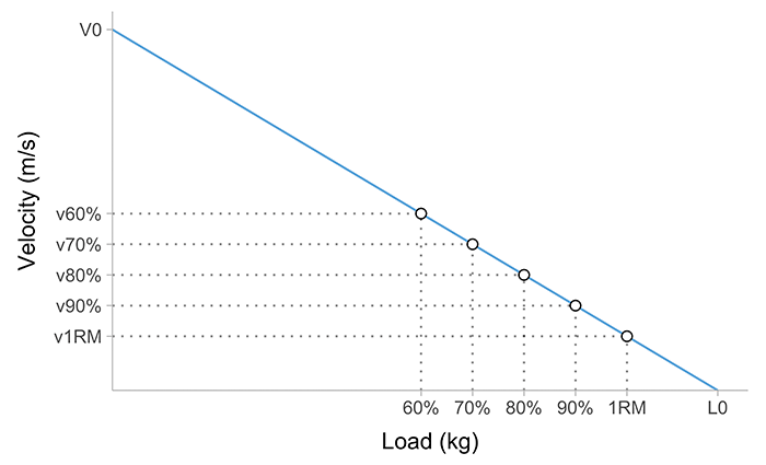
Figure 2: Velocity of sub-maximal loads. Loads are expressed using \(1RM\), in this case 60, 70, 80, and 90% \(1RM\).

Figure 1 and Figure 2 represents the LV profile and a first layer of the {LEVsim}. This layer can only generate single repetition velocities at different loads. But how do we simulate exertion effects, as in maximal number of repetitions that can be performed at certain load (i.e., Reps-Max relationship), and in reducing velocity of each repetition as one approaches failure point (i.e., Exertion-Velocity relationship)? But before I address that issue, I need to introduce another key concept.

Measurement Error

\(L_0\), \(V_0\), and \(v1RM\) represent theoretical latent constructs (i.e., DGP parameters) that cannot be directly measured, but are the causal mechanism behind the repetition velocities. In this theoretical model, repetition velocities are under the influence of another construct – measurement error. Measurement error is involved in all measurements and causes an measured score to be different from the true score (Allen and Yen 2001; Borsboom 2009; Jovanović 2020b; Novick 1966; Swinton et al. 2018). In plain English, given this theoretical LV profile (Figure 1 and Figure 2), one expects repetition velocity to be equal to Equation 2. But this doesn’t necessary need to be the case when we actually observe the repetition velocities. We thus need another set of parameters to simulate this phenomena.