[Playbook] Converting Just Jump to Smart Jump
Introduction
Coaches and athletes sometime change measurement/testing equipment. The problem is that the estimates from different equipment might differ (and they usually do). There are couple of soutions to this problem – (1) disregard the old scores (in which case coaches losses precious historical data) or (2) convert the old scores to the new and ideally maintain the measurement database with as little error as possible.
Since we are going for the second option, the practical question to be answered is how big is the error, or in other words signal vs. noise? I will present one way to evaluate the error of the conversion using Smallest Worthwihle Change metric.
Converting Just Jump to Smart Jump
Friend of mine, Sam Leahey is switching from Just Jump to Smart Jump contact mats and wants to convert the older Just Jump scores to the new Smart Jump scores.
We proposed the following protocol for data collection:
- Get couple of athletes (or all of them)
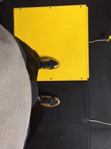
- Put mats close to each other and place left foot on one and right foot on another (see the picture)
- Perform the vertical jump and take the scores for each
- Switch the legs and perfom the jump again (this should remove any leg/differences)
- Randomize the start, to avoid any fatigue related issues
- Multiple athletes can repreat the procedure multiple times so we get as much data points as possible
Here is the picture of the procedure:
The data
The testing data was saved to .csv file. Let’s load it and show first couple of rows
# Load needed libraries
suppressPackageStartupMessages(library(reshape2))
suppressPackageStartupMessages(library(caret))
suppressPackageStartupMessages(library(dplyr))
suppressPackageStartupMessages(library(rethinking))
suppressPackageStartupMessages(library(boot))

# Load the data
jumpDataRaw <- read.csv("Jumps.csv",
                     header = TRUE,
                     stringsAsFactors = FALSE)

head(jumpDataRaw, 15)
## Attempt Date Name JJ.LEFT JJ.RIGHT SJ.RIGHT SJ.LEFT
## 1 1 17.3.16 Joe 23.8 24.3 18.56 19.65
## 2 2 21.3.16 Sam 19.0 17.1 13.87 12.56
## 3 3 21.3.16 Zach 12.5 12.8 10.80 8.40
## 4 4 21.3.16 Erik 14.2 15.4 11.31 11.31
## 5 5 24.3.16 Sam 19.9 20.7 14.82 16.30
## 6 6 24.3.16 Ashton 14.5 13.4 12.51 10.57
## 7 7 24.3.16 Jillian 17.1 16.7 11.69 11.69
## 8 8 25.3.16 Joe 22.5 24.6 17.61 19.22
## 9 9 25.3.16 Zach 13.7 13.6 8.89 10.98
## 10 10 25.3.16 Erik 16.1 14.3 10.56 12.26
## 11 11 25.3.16 AidanH 14.8 13.6 10.35 9.95
## 12 12 26.3.16 Ashton 15.4 16.7 11.59 11.97
## 13 13 26.3.16 Kara 10.9 12.7 7.38 9.86
## 14 14 28.3.16 Sam 19.3 20.4 14.29 15.96
## 15 15 30.3.16 Sam 19.9 18.4 14.82 14.23Let’s plot the JustJump left and right scores and SmartJump left and right scores (when left/right foot is placed on the mat).
# Just Jump
gg <- ggplot(jumpDataRaw, aes(x = JJ.LEFT, y = JJ.RIGHT)) +
      geom_smooth(method = "lm", color = "grey", alpha = 0.3) +
      geom_abline(slope = 1, color = "red", linetype = "dashed") +
      geom_point(color = "blue", alpha = 0.7) +
      theme_bw() +
      ggtitle("Just Jump leg difference scatterplot")
print(gg)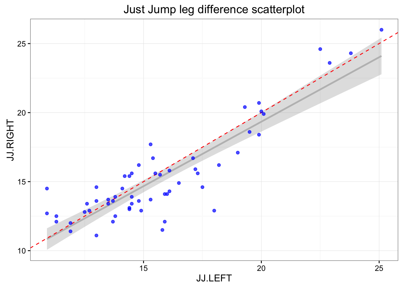
gg <- ggplot(jumpDataRaw, aes(x = JJ.LEFT - JJ.RIGHT)) +
      geom_density(fill = "blue", alpha = 0.3) +
      geom_histogram(aes(y=..density..), bins=20, alpha = 0.5) +
      geom_vline(xintercept = mean(jumpDataRaw$JJ.LEFT - jumpDataRaw$JJ.RIGHT),
                 color = "red", linetype = "dashed") +
      theme_bw() +
      ggtitle("Just Jump leg difference distribution")
print(gg)
# Smart Jump
gg <- ggplot(jumpDataRaw, aes(x = SJ.LEFT, y = SJ.RIGHT)) +
      geom_smooth(method = "lm", color = "grey", alpha = 0.3) +
      geom_abline(slope = 1, color = "red", linetype = "dashed") +
      geom_point(color = "blue", alpha = 0.7) +
      theme_bw() +
      ggtitle("Smart Jump leg difference scatterplot")
print(gg)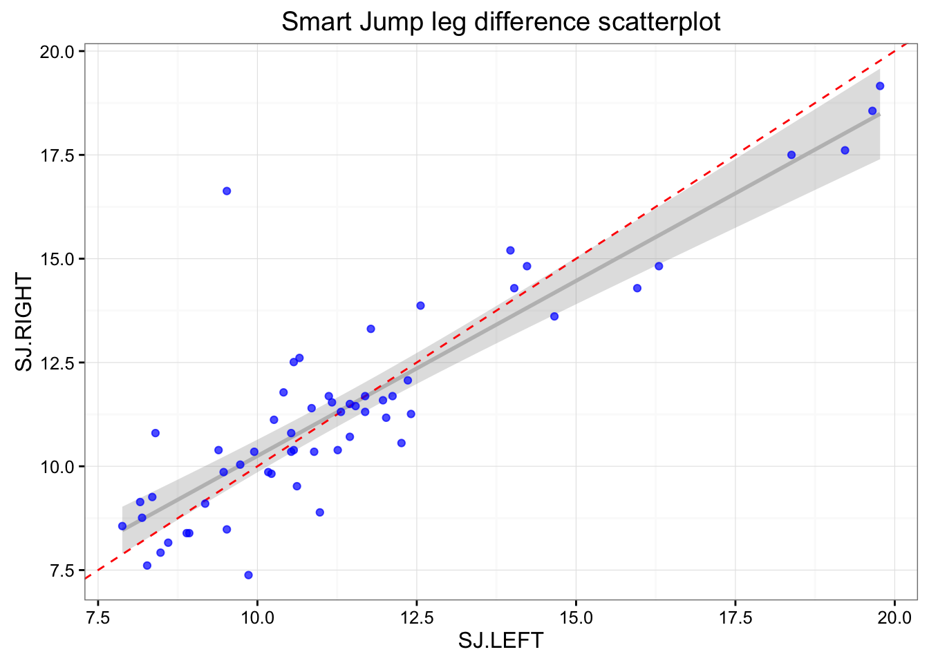
gg <- ggplot(jumpDataRaw, aes(x = SJ.LEFT - SJ.RIGHT)) +
      geom_density(fill = "blue", alpha = 0.3) +
      geom_histogram(aes(y=..density..), bins=20, alpha = 0.5) +
      geom_vline(xintercept = mean(jumpDataRaw$SJ.LEFT - jumpDataRaw$SJ.RIGHT),
                 color = "red", linetype = "dashed") +
      theme_bw() +
      ggtitle("Smart Jump leg difference distribution")
print(gg)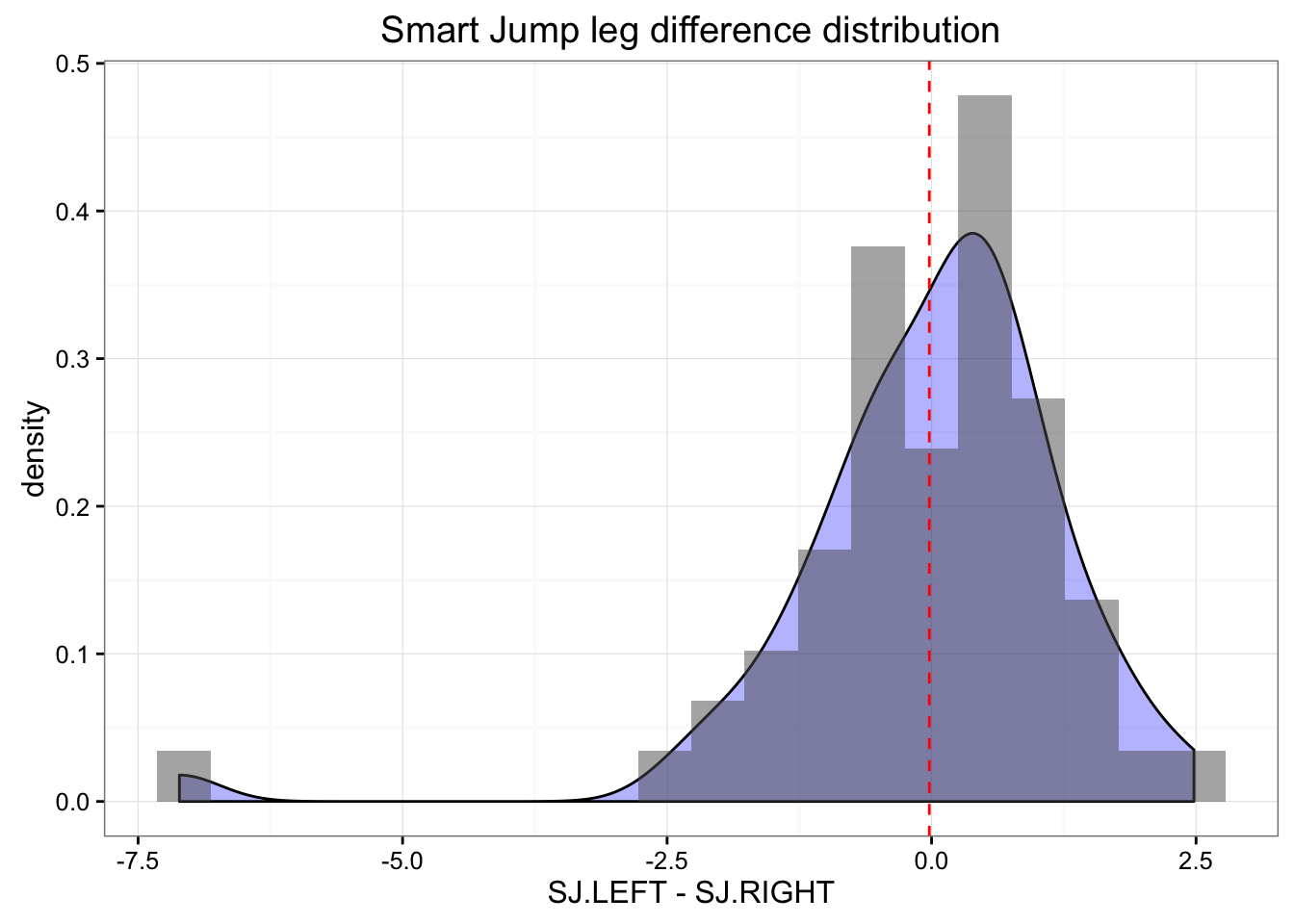
As can be seen there are differences in the left and right at each mat. This can be due numerous reasons: (1) measurement error, (2) typical error/variation, (3) change in the subjects states (i.e. fatigue, effort), (4) assymetrical landing/jumping.
Depending on the way the tests were done, change in subject states can be minimizied by athletes starting on different left/right position (randomization) or giving enough of rest between trial. Let’s assume that this was done.
In the Smart Jump there was clearly one outlier with big difference between jumps. Let’s find him and remove him
jumpDataRaw <- mutate(jumpDataRaw, JJ.Difference = JJ.LEFT - JJ.RIGHT)
jumpDataRaw <- mutate(jumpDataRaw, SJ.Difference = SJ.LEFT - SJ.RIGHT)

outlier <- which.min(jumpDataRaw$SJ.Difference)
print(jumpDataRaw[outlier,])
## Attempt Date Name JJ.LEFT JJ.RIGHT SJ.RIGHT SJ.LEFT JJ.Difference
## 24 25 5.4.16 AidanP 13.5 13.4 16.63 9.52 0.1
## SJ.Difference
## 24 -7.11We will remove this lad from the sample
jumpDataRaw <- jumpDataRaw[-outlier,]What is important to check is if there are correlations between SJ.Difference and JJ.Difference. If there is a correlation, that would imply that there was a change in athlete state between trials (either fatigue or change in effort) or there was assymmetry in landing (favoring one leg over the other).
Before plotting the relationship between two differences, we will normalize them them so they end up being on the same scale
jumpDataRaw$JJ.Difference <- as.numeric(scale(jumpDataRaw$JJ.Difference))
jumpDataRaw$SJ.Difference <- as.numeric(scale(jumpDataRaw$SJ.Difference))
Here is the plot
gg <- ggplot(jumpDataRaw, aes(x = SJ.Difference, y = JJ.Difference)) +
      geom_smooth(method = "lm", color = "grey", alpha = 0.3) +
      geom_abline(slope = -1, color = "red", linetype = "dashed") +
      geom_point(color = "blue", alpha = 0.7) +
      theme_bw() +
      ggtitle("Jump differences")
print(gg)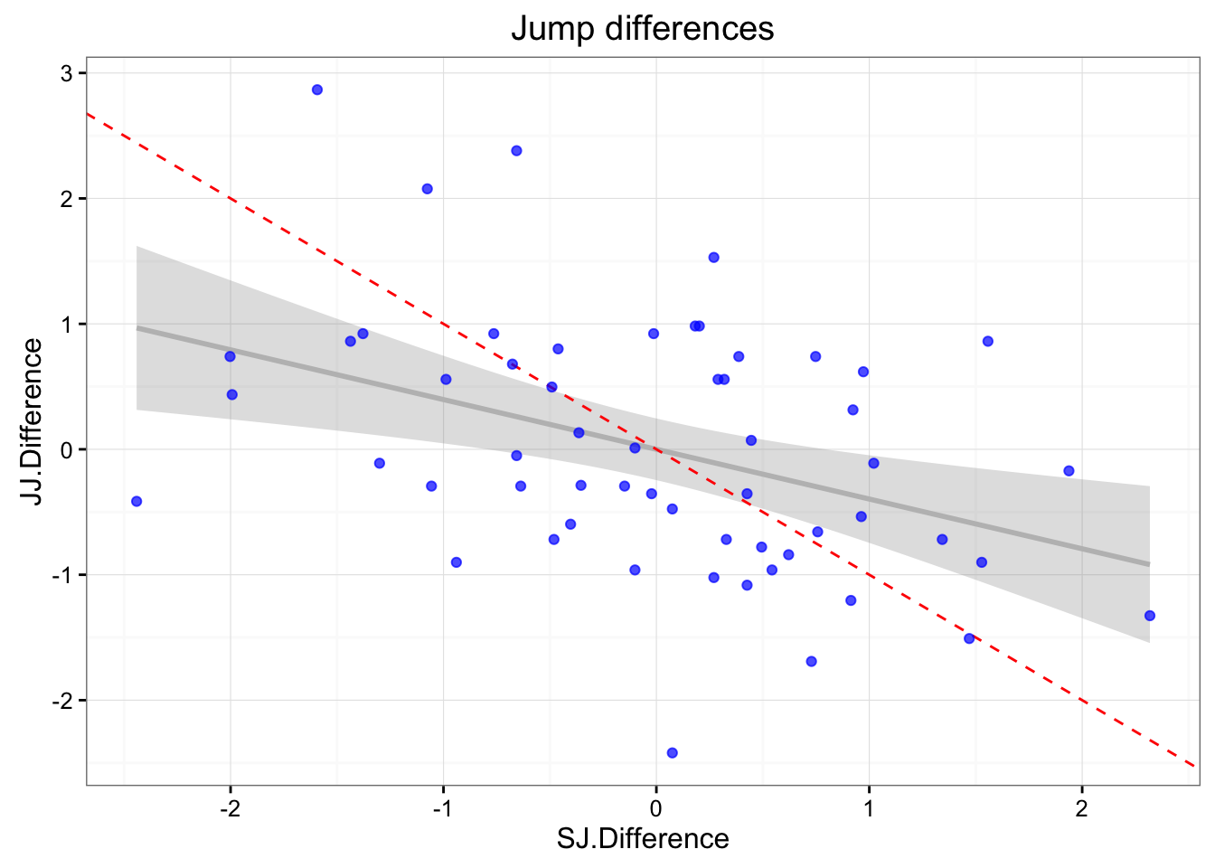
summary(lm(SJ.Difference ~ JJ.Difference, jumpDataRaw))##
## Call:
## lm(formula = SJ.Difference ~ JJ.Difference, data = jumpDataRaw)
##
## Residuals:
## Min 1Q Median 3Q Max
## -2.60580 -0.48194 -0.00346 0.57192 1.89890
##
## Coefficients:
## Estimate Std. Error t value Pr(>|t|)
## (Intercept) 3.220e-17 1.227e-01 0.000 1.00000
## JJ.Difference -3.965e-01 1.238e-01 -3.203 0.00226 **
## ---
## Signif. codes: 0 '***' 0.001 '**' 0.01 '*' 0.05 '.' 0.1 ' ' 1
##
## Residual standard error: 0.9263 on 55 degrees of freedom
## Multiple R-squared: 0.1572, Adjusted R-squared: 0.1419
## F-statistic: 10.26 on 1 and 55 DF, p-value: 0.002262cor(jumpDataRaw$SJ.Difference, jumpDataRaw$JJ.Difference)## [1] -0.3965054There appears to be negligable correlation between the two, so we will assume there were no change in athlete state between the trials.
Let’s inspect athletes that show highest “assymmetry”
jumpDataRaw <- mutate(jumpDataRaw, Assymmetry = sqrt(SJ.Difference^2 + JJ.Difference^2))
head(arrange(jumpDataRaw, desc(Assymmetry)), 10)
## Attempt Date Name JJ.LEFT JJ.RIGHT SJ.RIGHT SJ.LEFT
## 1 26 8.4.16 Alex 18.0 12.9 13.31 11.78
## 2 13 26.3.16 Kara 10.9 12.7 7.38 9.86
## 3 3 21.3.16 Zach 12.5 12.8 10.80 8.40
## 4 32 9.4.16 Christina 15.8 11.5 8.76 8.19
## 5 46 15.4.16 Erik 10.9 14.5 10.39 10.57
## 6 48 15.4.16 Ty 15.9 12.1 10.39 9.39
## 7 22 2.4.16 Ashton 16.5 14.9 12.61 10.66
## 8 8 25.3.16 Joe 22.5 24.6 17.61 19.22
## 9 6 24.3.16 Ashton 14.5 13.4 12.51 10.57
## 10 9 25.3.16 Zach 13.7 13.6 8.89 10.98
## JJ.Difference SJ.Difference Assymmetry
## 1 2.8666089 -1.59281546 3.279407
## 2 -1.3263223 2.31812911 2.670740
## 3 -0.4148155 -2.44132464 2.476315
## 4 2.3804719 -0.65652948 2.469348
## 5 -2.4201305 0.07494394 2.421291
## 6 2.0766363 -1.07590758 2.338802
## 7 0.7397597 -2.00244058 2.134716
## 8 -1.5086237 1.46961994 2.106117
## 9 0.4359241 -1.99268760 2.039812
## 10 -0.1717471 1.93776293 1.945359I will remove everyone who is above 2 for the further analysis
inconsistent <- jumpDataRaw$Assymmetry > 2
jumpDataRaw <-  jumpDataRaw[!inconsistent, ]
And here is the plot one more time with those lads removed.
jumpDataRaw <- mutate(jumpDataRaw, JJ.Difference = JJ.LEFT - JJ.RIGHT)
jumpDataRaw <- mutate(jumpDataRaw, SJ.Difference = SJ.LEFT - SJ.RIGHT)
jumpDataRaw$JJ.Difference <- as.numeric(scale(jumpDataRaw$JJ.Difference))
jumpDataRaw$SJ.Difference <- as.numeric(scale(jumpDataRaw$SJ.Difference))

gg <- ggplot(jumpDataRaw, aes(x = SJ.Difference, y = JJ.Difference)) +
      geom_smooth(method = "lm", color = "grey", alpha = 0.3) +
      geom_abline(slope = -1, color = "red", linetype = "dashed") +
      geom_point(color = "blue", alpha = 0.7) +
      theme_bw() +
      ggtitle("Jump differences")
print(gg)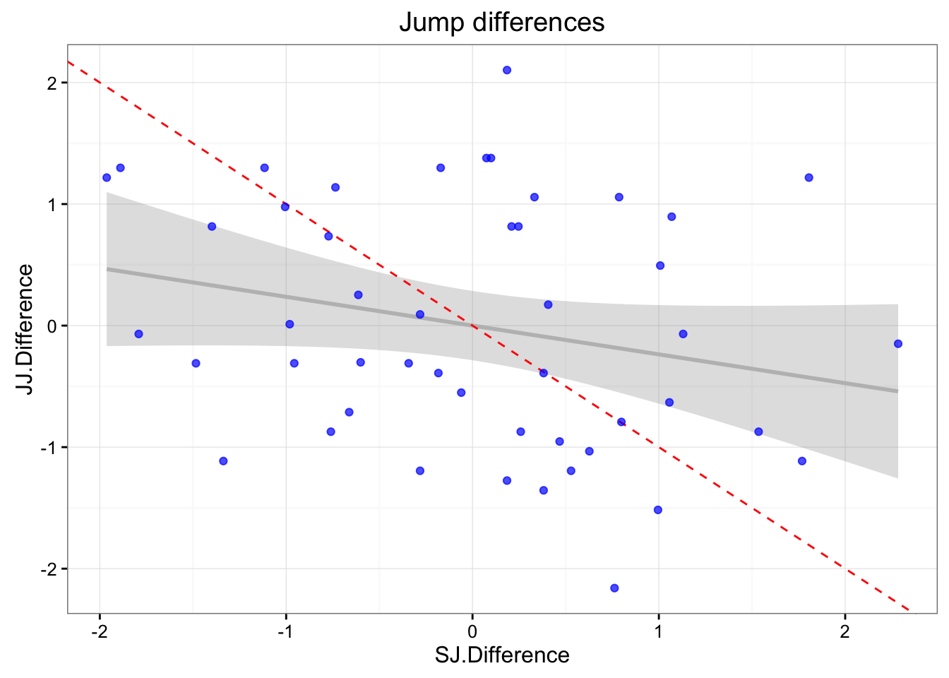
summary(lm(SJ.Difference ~ JJ.Difference, jumpDataRaw))##
## Call:
## lm(formula = SJ.Difference ~ JJ.Difference, data = jumpDataRaw)
##
## Residuals:
## Min 1Q Median 3Q Max
## -1.80747 -0.69757 0.09858 0.58990 2.24886
##
## Coefficients:
## Estimate Std. Error t value Pr(>|t|)
## (Intercept) -4.344e-17 1.417e-01 0.000 1.000
## JJ.Difference -2.368e-01 1.432e-01 -1.653 0.105
##
## Residual standard error: 0.9821 on 46 degrees of freedom
## Multiple R-squared: 0.0561, Adjusted R-squared: 0.03558
## F-statistic: 2.734 on 1 and 46 DF, p-value: 0.1051cor(jumpDataRaw$SJ.Difference, jumpDataRaw$JJ.Difference)## [1] -0.2368485SWC and TE
Let’s calculate Smallest Wortwhile Change (SWC) and Typical Error (TE) for each platform. Since couple of athletes repeated the test couple of times, the best we can do is to average them.
jumpDataAveraged <- jumpDataRaw %>%
                    select(3:7) %>%
                    group_by(Name) %>%
                    summarise_each(funs(mean)) %>%
                    ungroup()
To calculate SWC in a given test, we need to average them since we have two performed (left and right).
jumpDataAveraged <- mutate(jumpDataAveraged, JJ = (JJ.LEFT + JJ.RIGHT) / 2)
jumpDataAveraged <- mutate(jumpDataAveraged, SJ = (SJ.LEFT + SJ.RIGHT) / 2)
And to calculate TE we need to calculate the differences again:
jumpDataAveraged <- mutate(jumpDataAveraged, JJ.Difference = (JJ.LEFT - JJ.RIGHT))
jumpDataAveraged <- mutate(jumpDataAveraged, SJ.Difference = (SJ.LEFT - SJ.RIGHT))
And here is our averaged data that we will use for SWC and TE calculation (showing only first 5 rows):
head(as.data.frame(jumpDataAveraged))## Name JJ.LEFT JJ.RIGHT SJ.RIGHT SJ.LEFT JJ SJ
## 1 AidanH 14.35714 13.45714 10.06571 10.13714 13.90714 10.10143
## 2 AidanP 13.00000 14.10000 9.26000 9.62500 13.55000 9.44250
## 3 Amelia 16.00000 14.10000 11.45000 11.54000 15.05000 11.49500
## 4 Andrew 14.10000 14.50000 10.35000 10.53000 14.30000 10.44000
## 5 Ashley 17.20000 15.90000 11.69000 12.12000 16.55000 11.90500
## 6 Ashton 16.07500 15.92500 11.58000 11.42750 16.00000 11.50375
## JJ.Difference SJ.Difference
## 1 0.90 0.07142857
## 2 -1.10 0.36500000
## 3 1.90 0.09000000
## 4 -0.40 0.18000000
## 5 1.30 0.43000000
## 6 0.15 -0.15250000The SWC is calculate using between subjects standard deviation, multiplied by 0.2 (see Will Hopkins work). This is the smallest importance change in performance. Let’s calculate that for both JustJump and SmartJump
JJ.SWC <- 0.2 * sd(jumpDataAveraged$JJ)
SJ.SWC <- 0.2 * sd(jumpDataAveraged$SJ)
Here are the SWCs for our mats:
- JustJump SWC 0.63
- SmartJump SWC 0.52
Let’c calculate Typical Error/Variation for each. Here we are interested in the differences between two averaged trials (see Will Hopkins):
JJ.TE <- sd(jumpDataAveraged$JJ.Difference) / sqrt(2)
SJ.TE <- sd(jumpDataAveraged$SJ.Difference) / sqrt(2)
Here are the TEs for our mats:
- JustJump TE 0.61
- SmartJump TE 0.41
Let’s calculate signal to noise for each mat (this is SWC / TE).
- JustJump 1.03
- SmartJump 1.26
It seems that SmartJump has better signal to noise quality (i.e ability to discern smallest improvement in performance).
Conversion between mats
Let’s create the conversion between the mats. I will use average between left and right jumps for each mat, but will not summarise for each athlete to get more data points (trials) as I have done for SWC and TE calculation.
jumpData <- jumpDataRaw[3:7]
jumpData <- mutate(jumpData, JJ = (JJ.LEFT + JJ.RIGHT) / 2)
jumpData <- mutate(jumpData, SJ = (SJ.LEFT + SJ.RIGHT) / 2)
Let’s plot the data:
gg <- ggplot(jumpData, aes(x = JJ, y = SJ)) +
      geom_smooth(method = "lm", color = "grey", alpha = 0.3) +
      geom_point(color = "blue", alpha = 0.7) +
      theme_bw()
print(gg)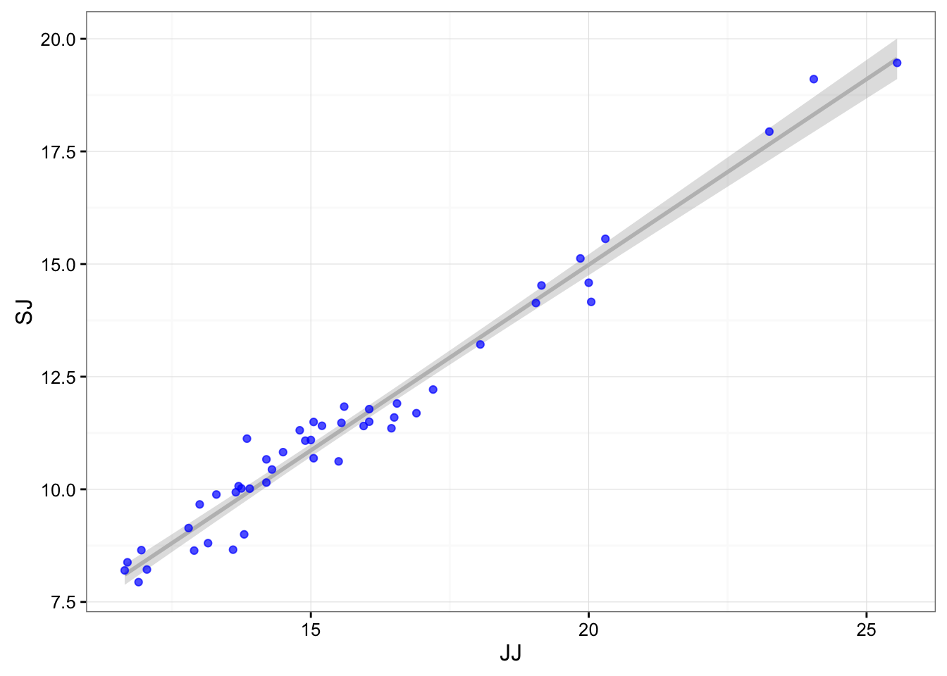
The simplest approach to conversion would be to use linear regression to get the formula:
linearModel <- lm(SJ ~ JJ, jumpData)
summary(linearModel)
##
## Call:
## lm(formula = SJ ~ JJ, data = jumpData)
##
## Residuals:
## Min 1Q Median 3Q Max
## -1.05121 -0.27433 0.09155 0.29789 1.20783
##
## Coefficients:
## Estimate Std. Error t value Pr(>|t|)
## (Intercept) -1.49285 0.34769 -4.294 8.98e-05 ***
## JJ 0.82383 0.02166 38.039 < 2e-16 ***
## ---
## Signif. codes: 0 '***' 0.001 '**' 0.01 '*' 0.05 '.' 0.1 ' ' 1
##
## Residual standard error: 0.4753 on 46 degrees of freedom
## Multiple R-squared: 0.9692, Adjusted R-squared: 0.9685
## F-statistic: 1447 on 1 and 46 DF, p-value: < 2.2e-16What we get is the following conversion formula:
SmartJump = -1.49 + 0.82 * JustJump
But we are also interested in the error of the model (in this case residual standard error or standard deviation of the residuals), which is equal to:
sd(residuals(linearModel))## [1] 0.4702623There is a slight difference between SD of residuals and residual standard error, becasue the latter is divided by degrees of freedom (N – 1 – k).
Prediction
Using residuals standard deviation (or RMSE – root mean square error, but this one is divided by N and not N – 1 as is in residuals standard error) we want to estimate how our model will generalize to the unseen data (because we will predict/convert for new athletes/trials).
Utilizing caret package I will evaluate our model performance (estiamted by RMSE) using repeated cross validation, or CV using 5 folds and 200 repeats.
ctr <- trainControl(method = "repeatedcv",
                    number = 5,
                    repeats = 200)

target = jumpData$SJ
predictors = select(jumpData, JJ)

model <- train(y = target,
               x = predictors,
               method = "lm",
               trControl = ctr)
print(model)
## Linear Regression
##
## 48 samples
## 1 predictor
##
## No pre-processing
## Resampling: Cross-Validated (5 fold, repeated 200 times)
## Summary of sample sizes: 36, 37, 39, 40, 40, 37, ...
## Resampling results
##
## RMSE Rsquared RMSE SD Rsquared SD
## 0.478878 0.9669502 0.09492898 0.02340058
##
## Using cross-validation of the simple linear regression, you can expect the following error (Root Mean Square Error; or residual standard deviation): 0.478878.
So here are our final model performance estimates (errors):
- Residual Standard Error = 0.4753464
- Residuals Standard Deviation = 0.4702623
- Training RMSE = 0.465338
- Cross-Validated RMSE = 0.478878
How big is the prediction error?
One way to compare prediction error (CV-RMSE) is to compare it to SWC of the target variable (SmartJump), which is 0.52. The ratio between the two can give you signal vs. noise estimate for comparing the SmartJump predictions (from JustJump scores) in detecting the SWC in the SmartJump performance. In this case the ration between CV-RMSE and SWC is 0.93, which is good. This mean that we can use the conversion from JustJump to SmartJump without loosing the ability to detect the SWC.
Bayesian computation
I recently started learning more about Bayesina Data Analysis, and will try to use it here. Bayesian data analysis is really flexible approach that can give us more “probabilistical” parameters (posteriors) and can “chew” a lot of things being thrown at it. In this case we can throw in SWC and TE, but this is still beyond my knowledge (might come back to this problem again in the next couple of months). For this reason I will use Bayesian approach to quantify to models ability to detect SWC in the target variable.
Please be free to let me know if I did any major/minor fuck ups here.
I will use rethinking package from the book I am reading (Statistical Rethinking – great book BTW)
Here is the definition of Bayesian model:
bayesianModel <- map(
        alist(
            SJ ~ dnorm(mu, sd), # Likelihood
            mu <- intercept + slope * JJ,
            slope ~ dnorm(1, 1), # Prior for slope
            intercept ~ dnorm(0, 1), # Prior for intercept
            sd ~ dunif(0, 1) # Prior for sigma (sd of residuals)
        ) , data = jumpData )
This is our data with 95% confidence interval and 95% prediction interval:
# Plot the model
JJ.seq <- seq(from = min(jumpData$JJ),
              to = max(jumpData$JJ),
              length.out = 100)

pred_dat <- data.frame(JJ = JJ.seq)

mu <- link(bayesianModel, data=pred_dat, 1e4)
FALSE [ 1000 / 10000 ]
[ 2000 / 10000 ]
[ 3000 / 10000 ]
[ 4000 / 10000 ]
[ 5000 / 10000 ]
[ 6000 / 10000 ]
[ 7000 / 10000 ]
[ 8000 / 10000 ]
[ 9000 / 10000 ]
[ 10000 / 10000 ]mu.mean <- apply(mu, 2, mean)
mu.PI <- apply(mu, 2, HPDI, prob = 0.95)
sim.SJ <- sim(bayesianModel, data = pred_dat, 1e4)FALSE [ 1000 / 10000 ]
[ 2000 / 10000 ]
[ 3000 / 10000 ]
[ 4000 / 10000 ]
[ 5000 / 10000 ]
[ 6000 / 10000 ]
[ 7000 / 10000 ]
[ 8000 / 10000 ]
[ 9000 / 10000 ]
[ 10000 / 10000 ]SJ.PI <- apply(sim.SJ, 2, HPDI, prob = 0.95)
# Plot the model
df <- data.frame(JJ.seq = JJ.seq,
SJ.mu = mu.mean,
SJ.CI.lower = mu.PI[1,],
SJ.CI.upper = mu.PI[2,],
SJ.PI.lower = SJ.PI[1,],
SJ.PI.upper = SJ.PI[2,])
gg <- ggplot(df, aes(x = JJ.seq, y = SJ.mu)) +
geom_line() +
geom_ribbon(aes(ymin = SJ.CI.lower, ymax = SJ.CI.upper),
fill = "grey", color = NA, alpha = 0.7) +
geom_ribbon(aes(ymin = SJ.PI.lower, ymax = SJ.PI.upper),
fill = "grey", color = NA, alpha = 0.4) +
geom_point(data = jumpData, aes(x = JJ, y = SJ), color = "blue", alpha = 0.5) +
theme_bw() +
xlab("JustJump") + ylab("SmartJump")
gg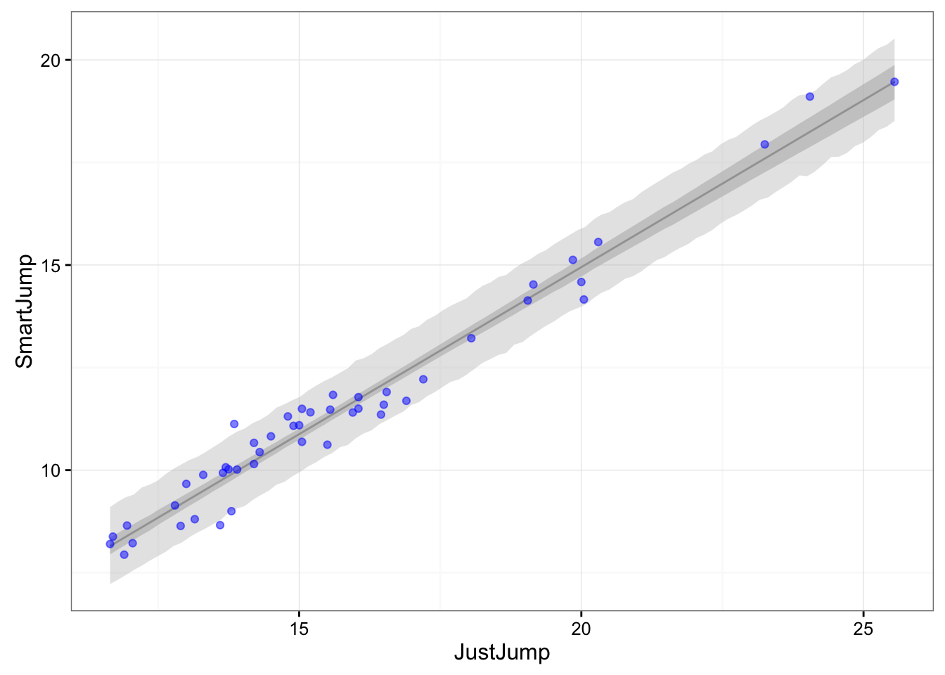
What we need to do next is to simulate the data points using the model parameters and calculate the residuals. We will draw 10,000 samples.
mu <- link(bayesianModel, data = jumpData, 1e4)FALSE [ 1000 / 10000 ]
[ 2000 / 10000 ]
[ 3000 / 10000 ]
[ 4000 / 10000 ]
[ 5000 / 10000 ]
[ 6000 / 10000 ]
[ 7000 / 10000 ]
[ 8000 / 10000 ]
[ 9000 / 10000 ]
[ 10000 / 10000 ]mu.mean <- apply(mu, 2, mean)
sim.SJ <- sim(bayesianModel, data = jumpData, 1e4)FALSE [ 1000 / 10000 ]
[ 2000 / 10000 ]
[ 3000 / 10000 ]
[ 4000 / 10000 ]
[ 5000 / 10000 ]
[ 6000 / 10000 ]
[ 7000 / 10000 ]
[ 8000 / 10000 ]
[ 9000 / 10000 ]
[ 10000 / 10000 ]modelResiduals <- t(sim.SJ) - mu.meanLet’s plot the distribution of the residuals over the SWC of the Smart Jump
gg <- ggplot(data.frame(Residuals = as.numeric(modelResiduals)),
             aes(x = Residuals)) +
      geom_vline(xintercept = -SJ.SWC, linetype = "longdash") +
      geom_vline(xintercept =  SJ.SWC, linetype = "longdash") +
      geom_density(fill = "blue", alpha = 0.5) +
      theme_bw()
print(gg)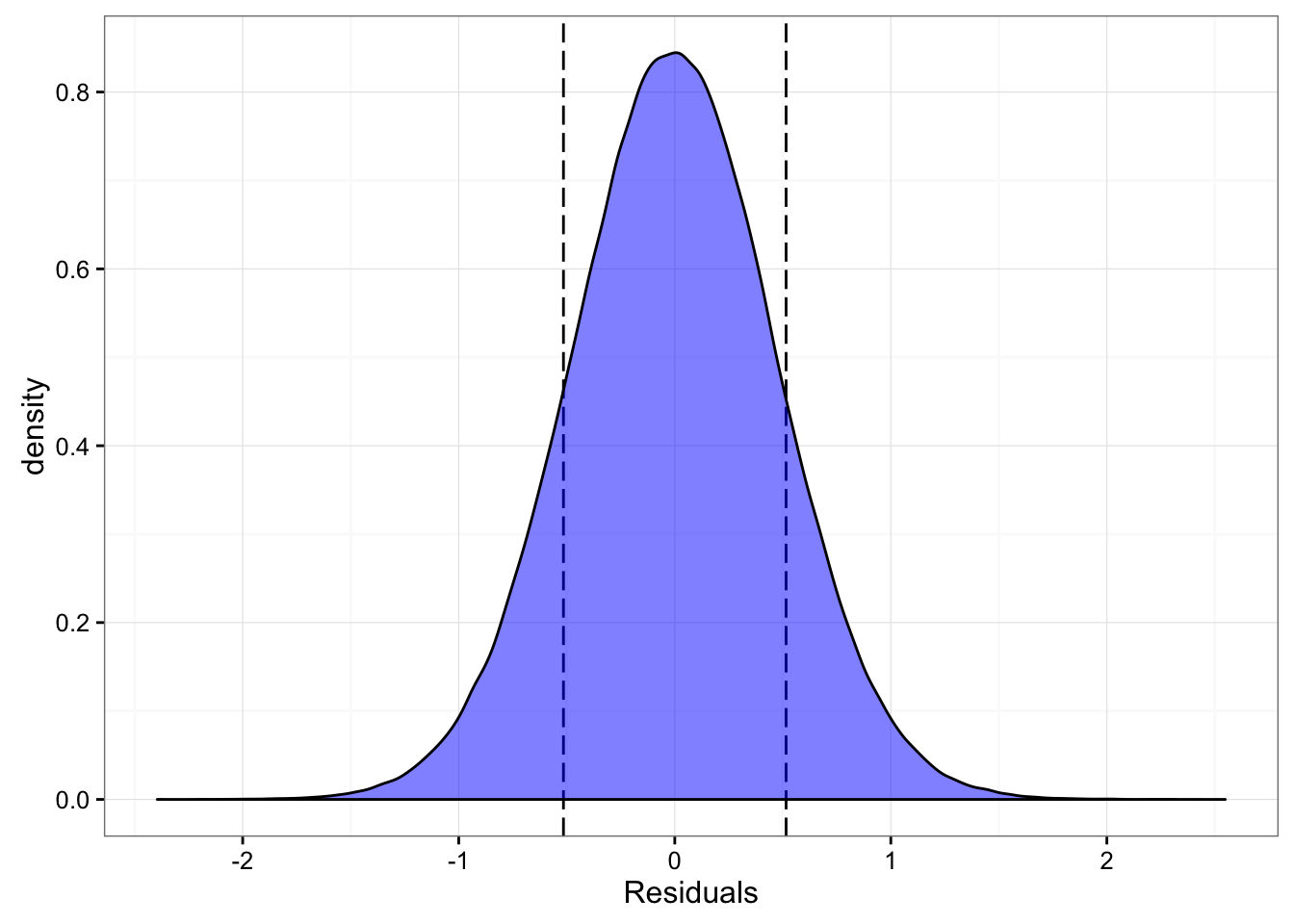
And we can easily calculate the probability of “capturing” SWC with converted jump height:
captured <- ifelse(modelResiduals < SJ.SWC & modelResiduals > -SJ.SWC, 1, 0)

SWCProbability <- sum(captured) / length(captured)
print(SWCProbability)
## [1] 0.7235458So the probability of capturing the SWC with converted model is 0.72. With the signal to noise ration of around 1 this is the percentage we an expect (based on normal distribution).
In the future I might add Typical Errors in the Bayesian model. That is currently beyond my knowledge. Besides we can plug in SWC in the Bayesian models itself and estimate this “capture” probabilistically (using the Bayesian model), rathen than with the method I’ve used here. There is a recent article that argues about this approach.
Bootstrap
We can also bootstrap our signal to noise ratio to get the idea of the distribution
signalToNoise <- function(data, i) {
    data2 <- data[i,]
    SWC <- sd(data2$SJ) * 0.2

    linearModel <- lm(SJ~JJ, data2)

    residualStandardError <- summary(linearModel)$sigma
    return(SWC / residualStandardError)
    }

stnBoot <- boot(jumpData, signalToNoise, R = 2000)
print(stnBoot)
##
## ORDINARY NONPARAMETRIC BOOTSTRAP
##
##
## Call:
## boot(data = jumpData, statistic = signalToNoise, R = 2000)
##
##
## Bootstrap Statistics :
## original bias std. error
## t1* 1.127203 0.02099104 0.1994454confint(stnBoot)## Bootstrap quantiles, type = bca
##
## 2.5 % 97.5 %
## 1 0.7844383 1.591124Above are our boostrapped signal-to-noise estimates and here is the distribution
df <- data.frame(SignalToNoise = stnBoot$t)
gg <- ggplot(df, aes(x = SignalToNoise)) +
      geom_density(fill = "blue", alpha = 0.3) +
      geom_histogram(aes(y=..density..), bins=20, alpha = 0.5) +
      geom_vline(xintercept = mean(df$SignalToNoise),
                 color = "red", linetype = "dashed") +
      theme_bw() +
      ggtitle("Distribution of the bootstrapped signal to noise ratio")
print(gg)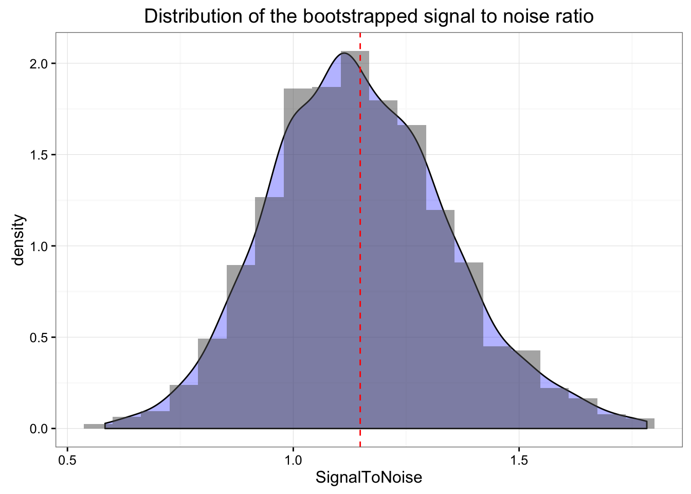
Conclusion
Please note that this was a playbook – let me know if I did any errors in the reasoning. In the near future I will use Bayesian approach to estimate signal to noise (and “capture” percentage) ratios using both SWC and TE in the model.



Responses