Load-Exertion Tables And Their Use For Planning – Part 4
Epley, or Not to Epley. That Is the Question
In the previous part, we have used a set of Epley’s equations to estimate both group/pooled and individual reps-max profiles, as well as to create progression tables (Equations 1). One characteristic of Epley’s equation is that 100% 1RM is achieved with 0RM, which is not an ecologically valid assumption. What the hell is 0RM in the first place? What we want is that 100% 1RM is associated with 1RM.
\[\begin{equation}
\begin{split}
nRM &= \frac{1 – \%1RM}{k \times \%1RM} \\
\%1RM &= \frac{1}{k \times nRM + 1}
\end{split}
\end{equation}\]
Equations 1
It is easy to check this feature by using Equations 2:
\[\begin{equation}
\begin{split}
nRM &= \frac{1 – \%1RM}{k \times \%1RM} \\
nRM &= \frac{1 – 1}{k \times 1} \\
nRM &= \frac{0}{k} \\
nRM &= 0 \\
\\
\%1RM &= \frac{1}{k \times nRM + 1} \\
\%1RM &= \frac{1}{k \times 0 + 1} \\
\%1RM &= \frac{1}{1} \\
\%1RM &= 1
\end{split}
\end{equation}\]
Equations 2
I am not sure why they selected this model definition in the first place. This feature of the Epley’s model is very confusing, which will be quite obvious later in this article series when I will introduce novel models and estimate 1RM alongside with the k parameter.
Luckily, this can be easily solved by using, what I call, Modified Epley’s (set of) Equations (Equations 3). I have renamed the k parameter to kmod to avoid confusion and to prevent using them interchangeably.
\[\begin{equation}
\begin{split}
nRM &= \frac{(kmod – 1) \times \%1RM + 1}{kmod \times \%1RM} \\
\%1RM &= \frac{1}{kmod \times (nRM – 1) + 1}
\end{split}
\end{equation}\]
Equations 3
Using this set of equations (Equations 3) correctly assumes that 1RM is achieved at 100% 1RM. I will leave you to check it out the same way we have done in Equation 2.
To demonstrate the difference between the two model definitions, I will again create a group/pooled model using our 12 athletes. The results are depicted in Figure 1. Estimated k is equal to 0.032, and estimated kmod is equal to 0.036.
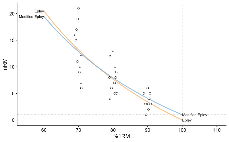
Figure 1: Group or pooled model fit using Epley (Equations 1) and Modified Epley (Equations 3) model definitions. This approach uses all the athletes to estimate the “average” profiles
Model performance is shown on Table 1 using five estimators: (1) mean-absolute-error (MAE), (2) root-mean-squared-error (RMSE), (3) maximal error (maxErr), (4) error interquartile range (IQR), and (5) variance explained (\(R^2\)) 4 . Since we are dealing with Group/pooled models, both models performed poorly. Please note that I have used Epley’s model to generated the data in the first place.
| Model | MAE (Reps) | RMSE (Reps) | maxErr (Reps) | IQR (Reps) | R2 |
|---|---|---|---|---|---|
| Epley | 2.30 | 3.02 | -7.82 | 3.76 | 0.63 |
| Modified Epley | 2.34 | 3.04 | -8.14 | 3.62 | 0.63 |
Table 1 – Group/Pooled model performance on the training data set. MAE = mean-absolute error; RMSE = root-mean-squared-error; maxErr = maximal error; IQR = error interquartile range; R2 = variance explained
Other model definitions, besides Epley and Modified Epley, can be used to model (or map out) max reps and %1RM relationship. The most common model used in data science is a simple linear regression (Equation 4).
\[\begin{equation}
nRM = slope \times \%1RM + intercept
\
\end{equation}\]
Equation 4
Simple linear regression is, simply put, a line. To estimate the best fit line through our observed data, we need to estimate two parameters: slope and intercept (Equation 4). This implies that we need at least three observations. When it comes to individual models, this implies that one needs to do three sets to fail. With Epley and Modified Epley model, one needs to do only two sets to failure. This is a practically meaningful difference.
Regression’s bigger brother, polynomial regression, particularly 2nd degree polynomial regression is also often utilized in modeling max reps and %1RM relationship (Equation 5).
\[\begin{equation}
nRM = slope_1 \times \%1RM + slope_2 \times \%1RM^2 + intercept
\end{equation}\]
Equation 5
Second degree polynomial have three parameters to be estimated: slope 1, slope 2 and intercept. The problem with this, particularly with the individual model, is that one needs at least four observations (i.e., sets to failure) for the parameters to be estimated. The additional problem involves different nRM associated with 100% 1RM (similar to the original Epley’s model), and for the polynomial model, we might have very weird predictions outside of observations range (i.e., predicting for 60% 1RM, when we have 70-90% observational data). Figure 2 depicts simple linear regression and 2nd-degree polynomial fit models. Note how the models behave around 100% 1RM.
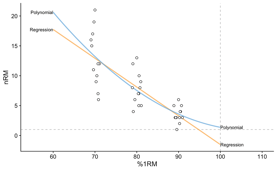
Figure 2 – Group or pooled model fit using simple linear regression (Equations 4) and polynomial regression (Equations 5) model definitions. This approach uses all the athletes to estimate the “average” profiles.
So what can we do about it? The benefit of a simple linear model is it’s simplicity (to be fair, Epley’s and Modified Epley’s models are not that complicated either), but we need to constrain them to have the origin at 1RM and 100% 1RM. The benefit of this, is that we also lose intercept parameter, and thus have only one parameter to estimate. Equations 6 represent model definitions that achieve exactly that. I have called this model definition Linear. Please note that I have used klin parameter name to differentiate it from slope, k, and kmod parameters.
\[\begin{equation}
\begin{split}
nRM &= (1 – \%1RM) \times klin + 1 \\
\%1RM &= \frac{klin – nRM + 1}{klin}
\end{split}
\end{equation}\]
Equations 6
Due to my own ignorance, I found out (a bit too late) that Brzycki’s equation (1 2 3) is the same as the Linear model proposed here. Estimated generic klin parameter in Brzycki’s research is equal to 36.
Using the Linear model (Equations 6), estimated klin parameter value is equal to 37.3. Figure 3 depicts model predictions for the Epley, Modified Epley, and Linear model. Make sure to note that the point of origin for the Modified Epley and Linear model is correctly 1RM and 100% 1RM.
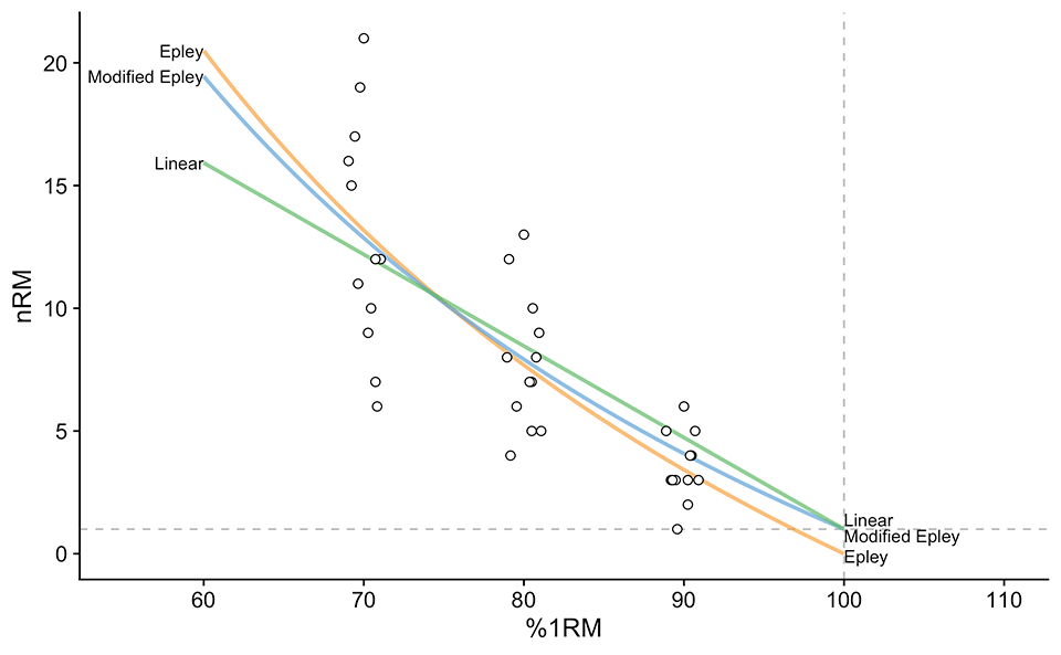
Figure 3 – Group or pooled model fit using Epley (Equations 1), Modified Epley (Equations 3), and Linear (Equations 6) model definitions. This approach uses all the athletes to estimate the “average” profiles
The benefit of the Linear model is in its simplicity, but it can be an ill-defined model for high-rep ranges. On the flip side, it can be good enough for the low rep ranges, which are in my opinion the most used ranges. Table 1.2 contains the performances of our three models: Epley, Modified Epley, and Linear. Please note that all three performed poorly, due to using all athletes to estimate the parameters (i.e., pooled).
| Model | MAE (Reps) | RMSE (Reps) | maxErr (Reps) | IQR (Reps) | R2 |
|---|---|---|---|---|---|
| Epley | 2.30 | 3.02 | -7.82 | 3.76 | 0.630 |
| Modified Epley | 2.34 | 3.04 | -8.14 | 3.62 | 0.630 |
| Linear | 2.50 | 3.19 | -8.81 | 3.17 | 0.623 |
Table 2 – Group/Pooled model performance on the training data set. MAE = mean-absolute error; RMSE = root-mean-squared-error; maxErr = maximal error; IQR = error interquartile range; R2 = variance explained
Table 3 contains estimated group/pooled reps-max tables using Epley, Modified Epley, and Linear model.
| Reps | 1 | 2 | 3 | 4 | 5 | 6 | 7 | 8 | 9 | 10 | 11 | 12 | 13 | 14 | 15 |
| Epley | 96.8 | 93.9 | 91.1 | 88.5 | 86 | 83.7 | 81.5 | 79.4 | 77.4 | 75.5 | 73.6 | 71.9 | 70.3 | 68.7 | 67.2 |
| Modified Epley | 100 | 96.5 | 93.3 | 90.2 | 87.4 | 84.7 | 82.2 | 79.8 | 77.6 | 75.5 | 73.5 | 71.6 | 69.8 | 68 | 66.4 |
| Linear | 100 | 97.3 | 94.6 | 92 | 89.3 | 86.6 | 83.9 | 81.2 | 78.6 | 75.9 | 73.2 | 70.5 | 67.8 | 65.2 | 62.5 |
Table 3 – Group/Pooled Reps-Max Tables using Epley, Modified Epley, and Linear model
Model equations summary, as well as default or generic parameter values for the Modified Epley and Linear model that are “compatible” with Epley’s k=0.0333 can be found in the Table 4. Please note that these are generic values (also value easy to remember), that can be used when you do not have any other information about the athlete (i.e. Bayesian prior). Table 5 contains reps-max tables using these default parameter values.
| Model | Predict nRM | Predict %1RM | Predict 1RM | Default parameter value |
|---|---|---|---|---|
| Epley | nRM = (1 – %1RM)/(k * %1RM) | %1RM = 1 / (k * nRM + 1) | 1RM = w * nRM * k + w | k = 0.0333 |
| Modifed Epley | nRM = ((kmod – 1) * %1RM + 1)/(kmod * %1RM) | %1RM = 1 / (kmod * (nRM – 1) + 1) | 1RM = w * (kmod * nRM – kmod + 1) | kmod = 0.0353 |
| Linear | nRM = (1 – %1RM) * klin + 1 | %1RM = (klin – nRM + 1) / klin | 1RM = w * klin / (klin – nRM + 1) | klin = 33, Brzycki = 36 |
Table 4 – Models definitions and their default/generic parameter values
| Reps | 1 | 2 | 3 | 4 | 5 | 6 | 7 | 8 | 9 | 10 | 11 | 12 | 13 | 14 | 15 |
| Epley | 96.8 | 93.8 | 90.9 | 88.2 | 85.7 | 83.3 | 81.1 | 79 | 76.9 | 75 | 73.2 | 71.4 | 69.8 | 68.2 | 66.7 |
| Modified Epley | 100 | 96.6 | 93.4 | 90.4 | 87.6 | 85 | 82.5 | 80.2 | 78 | 75.9 | 73.9 | 72 | 70.2 | 68.5 | 66.9 |
| Linear | 100 | 97 | 93.9 | 90.9 | 87.9 | 84.8 | 81.8 | 78.8 | 75.8 | 72.7 | 69.7 | 66.7 | 63.6 | 60.6 | 57.6 |
Table 5 – Generic Reps-Max Tables using the three models
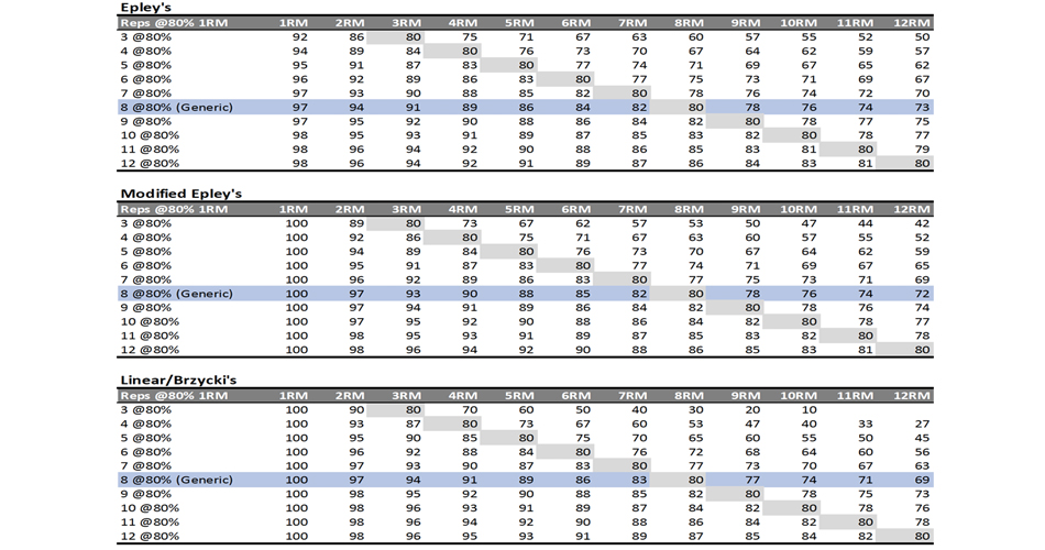
Similar to Epley’s model and equations, we can use these other two model definitions to create our progression tables. Table 1.6 contains all the equations used to implement all already explained progression tables/methods.
| Progression method | Epley | Modified Epley | Linear |
|---|---|---|---|
| Deducted Intensity | %1RM = 1 / (k * Reps + 1) – DI | %1RM = 1 / (kmod * (Reps – 1) + 1) – DI | %1RM = (klin – Reps + 1) / klin – DI |
| Relative Intensity | %1RM = RI / (k * Reps + 1) | %1RM = RI / (kmod * (Reps – 1) + 1) | %1RM = RI * (klin – Reps + 1) / klin |
| Reps In Reserve | %1RM = 1 / (k * (Reps + RIR) + 1) | %1RM = 1 / (kmod * (Reps + RIR – 1) + 1) | %1RM = (-RIR + klin – Reps + 1) / klin |
| %Max Reps | %1RM = %MR / (%MR + k * Reps) | %1RM = 1 / kmod * (Reps / %MR – 1) + 1) | %1RM = (klin – Reps / %MR + 1) / klin |
Table 6 – Equations used to implement different progression methods to Epley, Modified Epley, and Linear models
Multi-models and Multi-individuals
So far we have utilized group/pooled models (i.e., using all athletes in the data set pooled together) to get “average” profiles, average reps-max tables, and average progression tables. As explained in the previous part of this article series, we can fit individual models (we can also fit mixed-effects models when we have levels in our data, in this case, individual athletes), particularly for strength specialists using the small number of exercises. Figure 2.1 depicts Epley, Modified Epley, and Linear model fitted to individual data.
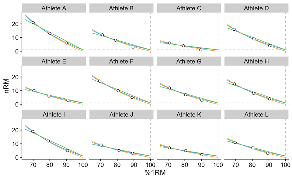
Figure 4 – Individual profiles using Epley, Modified Epley and Linear models
Table 7 contains individual model performances for each athlete and each model.
| Athlete | Model | est Param | MAE (Reps) | RMSE (Reps) | maxErr (Reps) | IQR (Reps) | R2 |
|---|---|---|---|---|---|---|---|
| Athlete A | Epley | 0.020 | 0.46 | 0.46 | -0.51 | 0.46 | 0.999 |
| Modified Epley | 0.021 | 0.20 | 0.21 | -0.27 | 0.24 | 0.999 | |
| Linear | 63.570 | 1.00 | 1.04 | 1.36 | 1.14 | 0.999 | |
| Athlete B | Epley | 0.034 | 0.22 | 0.28 | 0.46 | 0.31 | 0.998 |
| Modified Epley | 0.038 | 0.47 | 0.65 | 1.09 | 0.70 | 0.998 | |
| Linear | 34.980 | 0.97 | 1.11 | 1.68 | 1.28 | 1.000 | |
| Athlete C | Epley | 0.069 | 0.31 | 0.41 | 0.68 | 0.44 | 0.986 |
| Modified Epley | 0.089 | 0.56 | 0.78 | 1.31 | 0.83 | 0.986 | |
| Linear | 14.950 | 0.77 | 0.97 | 1.56 | 1.10 | 0.997 | |
| Athlete D | Epley | 0.028 | 0.30 | 0.32 | -0.45 | 0.37 | 0.998 |
| Modified Epley | 0.030 | 0.23 | 0.31 | 0.51 | 0.33 | 0.998 | |
| Linear | 45.710 | 0.97 | 1.01 | 1.35 | 1.10 | 0.999 | |
| Athlete E | Epley | 0.042 | 0.27 | 0.36 | -0.60 | 0.38 | 0.995 |
| Modified Epley | 0.048 | 0.23 | 0.26 | 0.37 | 0.31 | 0.995 | |
| Linear | 28.120 | 0.67 | 0.67 | 0.75 | 0.72 | 0.979 | |
| Athlete F | Epley | 0.025 | 0.30 | 0.34 | -0.51 | 0.41 | 0.997 |
| Modified Epley | 0.028 | 0.27 | 0.34 | 0.54 | 0.39 | 0.997 | |
| Linear | 49.350 | 1.00 | 1.07 | 1.48 | 1.20 | 1.000 | |
| Athlete G | Epley | 0.035 | 0.06 | 0.08 | 0.13 | 0.08 | 1.000 |
| Modified Epley | 0.039 | 0.46 | 0.51 | 0.78 | 0.56 | 1.000 | |
| Linear | 34.410 | 1.00 | 1.04 | 1.36 | 1.14 | 0.996 | |
| Athlete H | Epley | 0.030 | 0.17 | 0.23 | -0.40 | 0.23 | 0.999 |
| Modified Epley | 0.032 | 0.30 | 0.31 | 0.36 | 0.31 | 0.999 | |
| Linear | 42.170 | 1.06 | 1.06 | 1.11 | 1.07 | 0.989 | |
| Athlete I | Epley | 0.023 | 0.31 | 0.33 | -0.44 | 0.35 | 1.000 |
| Modified Epley | 0.024 | 0.11 | 0.15 | 0.25 | 0.15 | 1.000 | |
| Linear | 56.420 | 1.00 | 1.02 | 1.25 | 1.10 | 0.996 | |
| Athlete J | Epley | 0.046 | 0.17 | 0.23 | -0.39 | 0.25 | 0.998 |
| Modified Epley | 0.054 | 0.25 | 0.25 | 0.29 | 0.26 | 0.998 | |
| Linear | 24.670 | 0.67 | 0.67 | -0.67 | 0.67 | 0.988 | |
| Athlete K | Epley | 0.056 | 0.38 | 0.45 | -0.66 | 0.53 | 0.966 |
| Modified Epley | 0.068 | 0.37 | 0.43 | 0.59 | 0.51 | 0.966 | |
| Linear | 19.770 | 0.43 | 0.56 | 0.93 | 0.57 | 0.987 | |
| Athlete L | Epley | 0.038 | 0.37 | 0.42 | -0.65 | 0.49 | 0.985 |
| Modified Epley | 0.044 | 0.38 | 0.49 | 0.76 | 0.57 | 0.985 | |
| Linear | 31.140 | 0.67 | 0.84 | 1.34 | 0.94 | 0.997 |
Table 7: Individual models performance summary
Table 8 contains individual reps-max tables for each profile model. It is an extensive table, but it is important to understand this multi-model approach and how easy is to get lost in combinations and variations.
| Athlete | Model | 1 | 2 | 3 | 4 | 5 | 6 | 7 | 8 | 9 | 10 | 11 | 12 | 13 | 14 | 15 |
|---|---|---|---|---|---|---|---|---|---|---|---|---|---|---|---|---|
| Athlete A | Epley | 98.0 | 96.2 | 94.3 | 92.6 | 90.9 | 89.3 | 87.7 | 86.2 | 84.7 | 83.3 | 82.0 | 80.6 | 79.4 | 78.1 | 76.9 |
| Modified Epley | 100.0 | 97.9 | 95.9 | 94.0 | 92.1 | 90.4 | 88.7 | 87.0 | 85.4 | 83.9 | 82.4 | 81.0 | 79.6 | 78.3 | 77.0 | |
| Linear | 100.0 | 98.4 | 96.9 | 95.3 | 93.7 | 92.1 | 90.6 | 89.0 | 87.4 | 85.8 | 84.3 | 82.7 | 81.1 | 79.6 | 78.0 | |
| Athlete B | Epley | 96.7 | 93.6 | 90.7 | 88.0 | 85.5 | 83.0 | 80.8 | 78.6 | 76.6 | 74.6 | 72.8 | 71.0 | 69.3 | 67.7 | 66.2 |
| Modified Epley | 100.0 | 96.3 | 92.9 | 89.7 | 86.8 | 84.0 | 81.4 | 78.9 | 76.6 | 74.5 | 72.4 | 70.5 | 68.6 | 66.9 | 65.2 | |
| Linear | 100.0 | 97.1 | 94.3 | 91.4 | 88.6 | 85.7 | 82.8 | 80.0 | 77.1 | 74.3 | 71.4 | 68.5 | 65.7 | 62.8 | 60.0 | |
| Athlete C | Epley | 93.5 | 87.8 | 82.8 | 78.3 | 74.3 | 70.6 | 67.3 | 64.3 | 61.6 | 59.1 | 56.7 | 54.6 | 52.6 | 50.7 | 49.0 |
| Modified Epley | 100.0 | 91.9 | 84.9 | 79.0 | 73.8 | 69.3 | 65.3 | 61.7 | 58.5 | 55.6 | 53.0 | 50.6 | 48.5 | 46.5 | 44.6 | |
| Linear | 100.0 | 93.3 | 86.6 | 79.9 | 73.2 | 66.6 | 59.9 | 53.2 | 46.5 | 39.8 | 33.1 | 26.4 | 19.7 | 13.1 | 6.4 | |
| Athlete D | Epley | 97.3 | 94.8 | 92.4 | 90.1 | 87.9 | 85.8 | 83.8 | 81.9 | 80.1 | 78.4 | 76.8 | 75.2 | 73.6 | 72.2 | 70.8 |
| Modified Epley | 100.0 | 97.1 | 94.3 | 91.8 | 89.3 | 87.0 | 84.8 | 82.7 | 80.7 | 78.8 | 76.9 | 75.2 | 73.5 | 72.0 | 70.4 | |
| Linear | 100.0 | 97.8 | 95.6 | 93.4 | 91.2 | 89.1 | 86.9 | 84.7 | 82.5 | 80.3 | 78.1 | 75.9 | 73.7 | 71.6 | 69.4 | |
| Athlete E | Epley | 96.0 | 92.3 | 88.9 | 85.7 | 82.7 | 80.0 | 77.4 | 75.0 | 72.7 | 70.5 | 68.5 | 66.6 | 64.8 | 63.1 | 61.5 |
| Modified Epley | 100.0 | 95.4 | 91.3 | 87.4 | 83.9 | 80.7 | 77.7 | 74.9 | 72.3 | 69.9 | 67.6 | 65.5 | 63.5 | 61.6 | 59.9 | |
| Linear | 100.0 | 96.4 | 92.9 | 89.3 | 85.8 | 82.2 | 78.7 | 75.1 | 71.6 | 68.0 | 64.4 | 60.9 | 57.3 | 53.8 | 50.2 | |
| Athlete F | Epley | 97.5 | 95.2 | 92.9 | 90.8 | 88.7 | 86.8 | 84.9 | 83.1 | 81.4 | 79.7 | 78.1 | 76.6 | 75.2 | 73.7 | 72.4 |
| Modified Epley | 100.0 | 97.3 | 94.8 | 92.4 | 90.1 | 87.9 | 85.8 | 83.8 | 81.9 | 80.1 | 78.4 | 76.7 | 75.2 | 73.6 | 72.2 | |
| Linear | 100.0 | 98.0 | 95.9 | 93.9 | 91.9 | 89.9 | 87.8 | 85.8 | 83.8 | 81.8 | 79.7 | 77.7 | 75.7 | 73.7 | 71.6 | |
| Athlete G | Epley | 96.7 | 93.5 | 90.6 | 87.8 | 85.3 | 82.8 | 80.5 | 78.3 | 76.3 | 74.3 | 72.4 | 70.7 | 69.0 | 67.4 | 65.8 |
| Modified Epley | 100.0 | 96.3 | 92.8 | 89.6 | 86.6 | 83.7 | 81.1 | 78.6 | 76.3 | 74.1 | 72.0 | 70.1 | 68.2 | 66.4 | 64.8 | |
| Linear | 100.0 | 97.1 | 94.2 | 91.3 | 88.4 | 85.5 | 82.6 | 79.7 | 76.8 | 73.8 | 70.9 | 68.0 | 65.1 | 62.2 | 59.3 | |
| Athlete H | Epley | 97.1 | 94.4 | 91.9 | 89.4 | 87.1 | 85.0 | 82.9 | 80.9 | 79.0 | 77.2 | 75.5 | 73.8 | 72.3 | 70.8 | 69.3 |
| Modified Epley | 100.0 | 96.9 | 93.9 | 91.2 | 88.5 | 86.1 | 83.7 | 81.5 | 79.4 | 77.4 | 75.6 | 73.8 | 72.0 | 70.4 | 68.8 | |
| Linear | 100.0 | 97.6 | 95.3 | 92.9 | 90.5 | 88.1 | 85.8 | 83.4 | 81.0 | 78.7 | 76.3 | 73.9 | 71.5 | 69.2 | 66.8 | |
| Athlete I | Epley | 97.8 | 95.7 | 93.7 | 91.7 | 89.9 | 88.1 | 86.4 | 84.7 | 83.2 | 81.6 | 80.2 | 78.7 | 77.4 | 76.0 | 74.8 |
| Modified Epley | 100.0 | 97.6 | 95.4 | 93.2 | 91.2 | 89.2 | 87.4 | 85.6 | 83.8 | 82.2 | 80.6 | 79.0 | 77.5 | 76.1 | 74.7 | |
| Linear | 100.0 | 98.2 | 96.5 | 94.7 | 92.9 | 91.1 | 89.4 | 87.6 | 85.8 | 84.0 | 82.3 | 80.5 | 78.7 | 77.0 | 75.2 | |
| Athlete J | Epley | 95.6 | 91.5 | 87.8 | 84.3 | 81.1 | 78.2 | 75.4 | 72.9 | 70.5 | 68.3 | 66.2 | 64.2 | 62.3 | 60.6 | 58.9 |
| Modified Epley | 100.0 | 94.8 | 90.2 | 86.0 | 82.1 | 78.6 | 75.4 | 72.4 | 69.7 | 67.1 | 64.8 | 62.6 | 60.5 | 58.6 | 56.8 | |
| Linear | 100.0 | 95.9 | 91.9 | 87.8 | 83.8 | 79.7 | 75.7 | 71.6 | 67.6 | 63.5 | 59.5 | 55.4 | 51.4 | 47.3 | 43.2 | |
| Athlete K | Epley | 94.7 | 89.9 | 85.6 | 81.7 | 78.2 | 74.9 | 71.9 | 69.1 | 66.5 | 64.2 | 61.9 | 59.9 | 57.9 | 56.1 | 54.4 |
| Modified Epley | 100.0 | 93.6 | 88.0 | 83.1 | 78.6 | 74.7 | 71.1 | 67.8 | 64.8 | 62.1 | 59.6 | 57.3 | 55.1 | 53.1 | 51.3 | |
| Linear | 100.0 | 94.9 | 89.9 | 84.8 | 79.8 | 74.7 | 69.6 | 64.6 | 59.5 | 54.5 | 49.4 | 44.4 | 39.3 | 34.2 | 29.2 | |
| Athlete L | Epley | 96.3 | 92.9 | 89.7 | 86.7 | 83.9 | 81.2 | 78.8 | 76.5 | 74.3 | 72.2 | 70.3 | 68.4 | 66.7 | 65.0 | 63.4 |
| Modified Epley | 100.0 | 95.8 | 92.0 | 88.4 | 85.2 | 82.1 | 79.3 | 76.6 | 74.2 | 71.8 | 69.7 | 67.6 | 65.7 | 63.9 | 62.1 | |
| Linear | 100.0 | 96.8 | 93.6 | 90.4 | 87.2 | 83.9 | 80.7 | 77.5 | 74.3 | 71.1 | 67.9 | 64.7 | 61.5 | 58.3 | 55.0 |
Table 8 – Individual Reps-Max Tables
To finish this part of the article series, let’s explore how doing linear progression for the sets of 5 using normal variation/volume differs across our three archetypal athletes, which we have introduced in the previous part. Table 9 contains an example progression table for the sets of five reps (normal volume) using individual profiles of our three archetypal athletes estimated using Epley, Modified Epley, and Linear models. I have only included progression methods that have variable step increments (please refer to the previous part).
| Method | Model | Athlete | Step 1 | Step 2 | Step 3 | Step 4 | Step 2-1 Diff | Step 3-2 Diff | Step 4-3 Diff |
|---|---|---|---|---|---|---|---|---|---|
| Relative Intensity | Epley | Athlete A | 70.5 | 75.0 | 79.5 | 84.1 | 4.54 | 4.54 | 4.54 |
| Athlete B | 66.2 | 70.5 | 74.8 | 79.1 | 4.27 | 4.27 | 4.27 | ||
| Athlete C | 57.5 | 61.3 | 65.0 | 68.7 | 3.71 | 3.71 | 3.71 | ||
| Modified Epley | Athlete A | 71.4 | 76.0 | 80.6 | 85.2 | 4.61 | 4.61 | 4.61 | |
| Athlete B | 67.2 | 71.6 | 75.9 | 80.3 | 4.34 | 4.34 | 4.34 | ||
| Athlete C | 57.2 | 60.9 | 64.6 | 68.3 | 3.69 | 3.69 | 3.69 | ||
| Linear | Athlete A | 72.6 | 77.3 | 82.0 | 86.7 | 4.68 | 4.68 | 4.68 | |
| Athlete B | 68.6 | 73.1 | 77.5 | 81.9 | 4.43 | 4.43 | 4.43 | ||
| Athlete C | 56.8 | 60.4 | 64.1 | 67.8 | 3.66 | 3.66 | 3.66 | ||
| RIR 2 | Epley | Athlete A | 79.4 | 82.0 | 84.7 | 87.7 | 2.60 | 2.78 | 2.98 |
| Athlete B | 69.3 | 72.8 | 76.6 | 80.8 | 3.43 | 3.79 | 4.21 | ||
| Athlete C | 52.6 | 56.7 | 61.6 | 67.3 | 4.14 | 4.84 | 5.75 | ||
| Modified Epley | Athlete A | 79.6 | 82.4 | 85.4 | 88.7 | 2.80 | 3.00 | 3.23 | |
| Athlete B | 68.6 | 72.4 | 76.6 | 81.4 | 3.79 | 4.23 | 4.75 | ||
| Athlete C | 48.5 | 53.0 | 58.5 | 65.3 | 4.55 | 5.50 | 6.77 | ||
| Linear | Athlete A | 81.1 | 84.3 | 87.4 | 90.6 | 3.15 | 3.15 | 3.15 | |
| Athlete B | 65.7 | 71.4 | 77.1 | 82.8 | 5.72 | 5.72 | 5.72 | ||
| Athlete C | 19.8 | 33.1 | 46.5 | 59.9 | 13.38 | 13.38 | 13.38 | ||
| RIR Increment | Epley | Athlete A | 82.2 | 84.1 | 86.1 | 88.1 | 1.89 | 1.98 | 2.07 |
| Athlete B | 73.1 | 75.7 | 78.4 | 81.4 | 2.57 | 2.75 | 2.96 | ||
| Athlete C | 57.1 | 60.4 | 64.1 | 68.2 | 3.26 | 3.66 | 4.13 | ||
| Modified Epley | Athlete A | 82.7 | 84.7 | 86.9 | 89.1 | 2.04 | 2.14 | 2.25 | |
| Athlete B | 72.8 | 75.6 | 78.7 | 82.1 | 2.86 | 3.10 | 3.36 | ||
| Athlete C | 53.5 | 57.2 | 61.4 | 66.3 | 3.69 | 4.24 | 4.92 | ||
| Linear | Athlete A | 84.6 | 86.7 | 88.8 | 91.0 | 2.15 | 2.15 | 2.15 | |
| Athlete B | 71.9 | 75.8 | 79.7 | 83.6 | 3.90 | 3.90 | 3.90 | ||
| Athlete C | 34.3 | 43.5 | 52.6 | 61.7 | 9.12 | 9.12 | 9.12 | ||
| %MR Step Const | Epley | Athlete A | 83.3 | 85.7 | 87.5 | 88.9 | 2.38 | 1.79 | 1.39 |
| Athlete B | 74.6 | 77.9 | 80.4 | 82.5 | 3.30 | 2.54 | 2.02 | ||
| Athlete C | 59.1 | 63.4 | 66.9 | 69.8 | 4.33 | 3.50 | 2.89 | ||
| Modified Epley | Athlete A | 83.9 | 86.5 | 88.4 | 89.9 | 2.58 | 1.94 | 1.51 | |
| Athlete B | 74.5 | 78.2 | 81.0 | 83.3 | 3.70 | 2.87 | 2.30 | ||
| Athlete C | 55.6 | 60.6 | 64.8 | 68.3 | 4.98 | 4.14 | 3.50 | ||
| Linear | Athlete A | 85.8 | 88.5 | 90.3 | 91.7 | 2.62 | 1.87 | 1.40 | |
| Athlete B | 74.3 | 79.0 | 82.4 | 85.0 | 4.76 | 3.40 | 2.55 | ||
| Athlete C | 39.8 | 51.0 | 58.9 | 64.9 | 11.15 | 7.96 | 5.97 | ||
| %MR Step Var | Epley | Athlete A | 81.3 | 84.3 | 86.4 | 88.0 | 2.93 | 2.13 | 1.62 |
| Athlete B | 72.0 | 75.9 | 78.9 | 81.2 | 3.97 | 2.99 | 2.33 | ||
| Athlete C | 55.7 | 60.7 | 64.7 | 68.0 | 5.01 | 3.99 | 3.26 | ||
| Modified Epley | Athlete A | 81.8 | 84.9 | 87.2 | 89.0 | 3.16 | 2.31 | 1.77 | |
| Athlete B | 71.5 | 75.9 | 79.3 | 81.9 | 4.42 | 3.36 | 2.64 | ||
| Athlete C | 51.9 | 57.6 | 62.2 | 66.1 | 5.66 | 4.65 | 3.89 | ||
| Linear | Athlete A | 83.5 | 86.9 | 89.2 | 90.9 | 3.36 | 2.30 | 1.68 | |
| Athlete B | 70.1 | 76.2 | 80.4 | 83.4 | 6.11 | 4.19 | 3.05 | ||
| Athlete C | 30.1 | 44.3 | 54.1 | 61.3 | 14.29 | 9.80 | 7.14 |
Table 9 – Example progression table for the sets of five reps (normal volume) using individual profiles of our three archetypal athletes estimated using Epley, Modified Epley, and Linear models.
Please note that all of these models and progression tables are very easily produced using the strengthPro web app.
In the next part of this article series, I will explain how you can avoid direct 1RM testing and doing reps to failure by using a novel approach. Stay tuned!
References
- Brzycki, Matt. 1991. A Practical Approach to Strength Training. Rev. ed. Grand Rapids, Mich: Masters Press
- Matt Brzycki 1993. “Strength Testing—Predicting a One-Rep Max from Reps-to-Fatigue” Journal of Physical Education, Recreation & Dance 64 (1): 88–90. https://doi.org/10.1080/07303084.1993.10606684
- DiStasio, Thomas J. 2014. “Validation of the Brzycki and Epley Equations for the 1 Repetition Maximum Back Squat Test in Division I College Football Players,” 40
- Jovanović, Mladen. 2020. Bmbstats: Bootstrap Magnitude-based Statistics for Sports Scientists. Mladen Jovanović


Responses